Category Archives: Statistics

Incanter blog post roundup

There have been several cool blog posts over the last few weeks featuring Incanter that I would like to highlight here.

Working with R from Clojure and Incanter

Joel Boehland has introduced Rincanter, which lets you use R from Clojure and Incanter. This is fantastically cool, as it opens up the vast number of R libraries to Clojure/Incanter, translating between R and Clojure data types, including Incanter datasets.

Check out Joel’s latest blog post, All your datasets R belong to us (I love that name), where he introduces Rincanter and demonstrates its use.

Working with data sets in Clojure with Incanter and MongoDB

This post will cover some new dataset functionality I’ve recently added to Incanter, including the use of MongoDB as a back-end data store for datasets.

Basic dataset functionality

First, load the basic Incanter libraries

(use '(incanter core stats charts io))

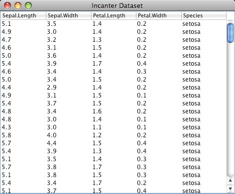
Next load some CSV data using the incanter.io/read-dataset function, which takes a string representing either a filename or a URL to the data.

(def data
  (read-dataset
    "http://github.com/liebke/incanter/raw/master/data/cars.csv"
     :header true))

The default delimiter is \, but a different one can be specified with the :delim option (e.g. \tab). The cars.csv file is a small sample data set that is included in the Incanter distribution, and therefore could have been loaded using get-dataset,

(incanter.datasets/get-dataset :cars)

See the documentation for get-dataset for more information on the included sample data.

We can get some information on the dataset, like the number of rows and columns using either the dim function or the nrow and ncol functions, and we can view the columns names with the col-names function.

user> (dim data)
[50 2]
user> (col-names data)
["speed" "dist"]

We can see that there are just 50 rows and two columns and that the column names are “speed” and “dist”. The data are 50 observations, from the 1920s, of automobile breaking distances observed at different speeds.

I will use Incanter’s new with-data macro and $ column-selector function to access the dataset’s columns. Within the body of a with-data expression, columns of the bound dataset can be accessed by name or index, using the $ function, for instance ($ :colname) or ($ 0).

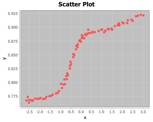
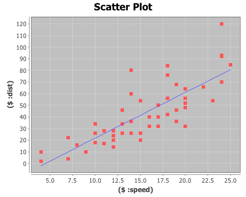
For example, the following code will create a scatter plot of the data (speed vs. dist), and then add a regression line using the fitted values returned from the incanter.stats/linear-model function.

(with-data data
  (def lm (linear-model ($ :dist) ($ :speed)))
  (doto (scatter-plot ($ :speed) ($ :dist))
    (add-lines ($ :speed) (:fitted lm))
    view))

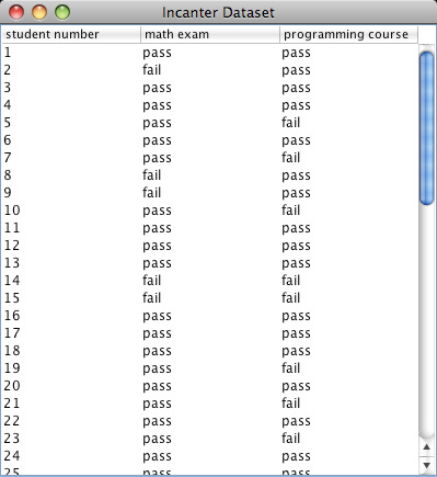
Within the with-data expression, the dataset itself is bound to $data, which can be useful if you want to perform operations on it. For instance, the following code uses the conj-cols function to prepend an integer ID column to the dataset, and then displays it in a window.

(with-data (get-dataset :cars)
  (view (conj-cols (range (nrow $data)) $data)))

The conj-cols function returns a dataset by conjoining sequences together as the columns of the dataset, or by prepending/appending columns to an existing dataset, and the related conj-rows function conjoins rows.

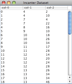
We can create a new dataset that adds the fitted (or predicted values) to the original data using the conj-cols function.

(def results (conj-cols data (:fitted lm)))

You’ll notice that the column names are changed to generic ones (i.e. col-0, col-1, col-2), this is done to prevent naming conflicts when merging datasets. We can add more meaningful names with the col-names function.

(def results (col-names data [:speed :dist :predicted-dist]))

We could have used the -> (thread) macro to perform both steps, as well as add the residuals from the output of linear-model to the dataset

(def results (-> (conj-cols data (:fitted lm) (:residuals lm))
                 (col-names [:speed :dist :predicted :residuals])))

Querying data sets with the $where function

Another new function, $where, lets you query an Incanter dataset using a syntax based on MongoDB and Somnium’s Congomongo Clojure library.

To perform a query, pass a query-map to the $where function. For instance, to get the rows from the results data set where the value of speed is 10, use

($where {:speed 10} results)

For the rows where the speed is between 10 and 20, use

($where {:speed {:$gt 10 :$lt 20}} results)

For rows where the speed is in the set #{4 7 24 25}, use

($where {:speed {:$in #{4 7 24 25}}} results)

Or not in that set,

($where {:speed {:$nin #{4 7 24 25}}} results)

Like the $ function, $where can be used within with-data, where the dataset is passed implicitly. For example, to get the mean speed of the observations that have residuals between -10 and 10 from the results dataset,

(with-data results
  (mean ($ :speed ($where {:residuals {:$gt -10 :$lt 10}}))))

which returns 14.32.

Query-maps don’t support ‘or’ directly, but we can use conj-rows to construct a dataset where speed is either less than 10 or greater than 20 as follows:

(with-data results
  (conj-rows ($where {:speed {:$lt 10}})
             ($where {:speed {:$gt 20}})))

An alternative to conjoining query results is to pass $where a predicate function that accepts a map containing the key/value pairs of a row and returns a boolean indicating whether the row should be included. For example, to perform the above query we could have done this,

(with-data results
  ($where (fn [row] (or (< (:speed row) 10) (> (:speed row) 20)))))

Storing and Retrieving Incanter datasets in MongoDB

The new incanter.mongodb library can be used with Somnium’s Congomongo to store and retrieve datasets in a MongoDB database.

MongoDB is schema-less, document-oriented database that is well suited as a data store for Clojure data structures. Getting started with MongoDB is easy, just download and unpack it, and run the following commands (on Linux or Mac OS X),

$ mkdir -p /data/db
$ ./mongodb/bin/mongod &

For more information, see the MongoDB quick start guide.

Once the database server is running, load Incanter’s MongoDB library and Congomongo,

(use 'somnium.congomongo)
(use 'incanter.mongodb)

and use Congomongo’s mongo! function to connect to the “mydb” database on the server running on the localhost on the default port.

(mongo! :db "mydb")

If mydb doesn’t exist, it will be created. Now we can insert the results dataset into the database with the incanter.mongodb/insert-dataset function.

(insert-dataset :breaking-dists results)

The first argument, :breaking-dists, is the name the collection will have in the database. We can now retrieve the dataset with the incanter.mongodb/fetch-dataset function.

(def breaking-dists (fetch-dataset :breaking-dists))

Take a look at the column names of the retrieved dataset and you’ll notice that MongoDB added a couple, :_ns and :_id, in order to uniquely identify each row.

user> (col-names breaking-dists)
[:speed :_ns :_id :predicted :residuals :dist]

The fetch-dataset function (and the congomongo.fetch function that it’s based on) support queries with the :where option. The following example retrieves only the rows from the :breaking-dists collection in the database where the :speed is between 10 and 20 mph, and then calculates the average breaking distance of the resulting observations.

(with-data (fetch-dataset :breaking-dists
			  :where {:speed {:$gt 10 :$lt 20}})
  (mean ($ :dist)))

The syntax for Congomongo’s query-maps is nearly the same as that for the $where function, although :$in and :$nin take a Clojure vector instead of a Clojure set.

For more information on the available functionality in Somnium’s Congomongo, visit its Github repository or read the documentation for incanter.mongodb

(doc incanter.mongodb)

The complete code for this post can be found here.

Chi-square goodness-of-fit, Benford’s law, and the Iranian election

Benford’s law has been discussed as a means of analyzing the results of the 2009 Iranian election by several analysts. One of the first attempts was in a paper (pdf) by Boudewijn Roukema, where he concluded that the data did not follow Benford’s law, and that there was evidence for vote tampering. Andrew Gelman responded; he was not convinced by the statistics of this particular analysis (his criticism was of the statistical analysis, and didn’t reflect his opinion of the possibility of vote tampering).

Stochastic Democracy and the Daily Kos also used Benford’s law to analyze the election data, here, but came to the opposite conclusion of Roukema; the data did follow Benford’s law. A third analysis was performed by John Graham-Cumming in this blog post. He came to the same conclusion as Stochastic Democracy and Daily Kos, that the data did follow Benford’s law. His analysis is based on this data, available from the Guardian’s Data Blog.

Again, like Gelman, I’m not convinced that Benford’s law can necessarily be used to draw conclusions on the presence or absence of vote tampering, but it is an interesting example of a Chi-square goodness-of-fit analysis, comparing some real-world data with a theoretical distribution, Benford’s law in this case. So I will demonstrate how to perform the analysis with Incanter using the data set made available by the Guardian. A CSV file with the data can be found here.

First load the necessary libraries,

(use '(incanter core stats charts io))

and read the data using the read-dataset function.

(def votes (read-dataset "data/iran_election_2009.csv" 
                         :header true))

Now, create variables representing the regions and the candidates.

(def regions (sel votes :cols "Region"))
(def ahmadinejad-votes (sel votes :cols "Ahmadinejad"))
(def mousavi-votes (sel votes :cols "Mousavi"))
(def rezai-votes (sel votes :cols "Rezai"))
(def karrubi-votes (sel votes :cols "Karrubi"))

We need to write a small function that will take a number and return only the first digit. We can do that by converting the number into a string with the str function, taking the first character of the string, and then converting that character into a number again.

(defn first-digit [x] 
  (Character/digit (first (str x)) 10)) 

Now, map the first-digit function over the vote counts in each of the 30 regions for each candidate.

(def ahmadinejad (map first-digit ahmadinejad-votes))
(def mousavi (map first-digit mousavi-votes))
(def rezai (map first-digit rezai-votes))
(def karrubi (map first-digit karrubi-votes))

Now we have a list of first-digits across the different regions, for each candidate. Next, define function that implements Benford’s Law, create a variable containing the probabilities for each of the nine digits, and calculate the expected frequencies for the 30 regions.

(defn benford-law [d] (log10 (plus 1 (div d))))
(def benford-probs (benford-law (range 1 11)))
(def benford-freq (mult benford-probs (count regions)))

We will then need a function that takes the list of first digits for each candidate and returns the counts for each digit. We can use the :counts field returned by the tabulate function to do most of the work.

(defn get-counts [digits] 
  (map #(get (:counts (tabulate digits)) % 0) 
       (range 1.0 10.0 1.0)))

It’s always a good idea to look at the data, so plot the predicted first-digit frequencies and the frequencies for Ahmadinejad and Mousavi.

(doto (xy-plot (range 1 10) (get-counts ahmadinejad)
               :legend true :series-label "Ahmadinejad"
               :y-label "First digit frequency"
               :x-label "First digit"
               :title "First digit frequency by candidate")
      (add-lines (range 1 10) (get-counts mousavi) 
                 :series-label "Mousavi")
      (add-lines (range 1 10) benford-freq 
                 :series-label "Predicted")
      clear-background
      view)

Based on that plot, the digit frequencies look like they follow Benford’s law. We can confirm that with a Chi-square goodness-of-fit test using the chisq-test function. Start with Ahmadinejad,

(def ahmadinejad-test 
  (chisq-test :table (get-counts ahmadinejad) 
              :probs benford-probs))
(:X-sq ahmadinejad-test)
(:p-value ahmadinejad-test)

The X-square test value is 5.439 with a p-value of 0.71. Based on these values we cannot reject the null hypothesis that the observed distribution of first-digits is the same as the expected distribution, which follows Benford’s law. Next test Mousavi’s vote counts,

(def mousavi-test 
  (chisq-test :table (get-counts mousavi) 
              :probs benford-probs))
(:X-sq mousavi-test) 
(:p-value mousavi-test)

The X-square test value for Mousavi is 5.775 with a p-value of 0.672. Like Ahmadinejad, we cannot reject the null hypothesis. We might as well test the distributions of first-digits for the remaining two candidates (which we didn’t plot), Rezai and Karrubi.

(def rezai-test 
  (chisq-test :table (get-counts rezai) 
              :probs benford-probs))
(:X-sq rezai-test) 
(:p-value rezai-test) 

The X-square test value for Rezai is 12.834 with a p-value of 0.118, so we can’t reject the null hypothesis.

(def karrubi-test 
  (chisq-test :table (get-counts karrubi) 
              :probs benford-probs))
(:X-sq karrubi-test) 
(:p-value karrubi-test) 

Karrubi’s X-square value is 8.8696 with a p-value of 0.353, and like the other candidates appears to follow Benford’s law.

The conclusion based on the vote count summaries for the 30 Iranian regions, is that the votes follow Benford’s law.

Last-digit frequencies

Another approach to identifying vote tampering is to examine the last digit of the vote counts, instead of the first. This approach was discussed in this Washington Post article.

Unlike first-digits, last-digits don’t follow Benford’s law, but rather follow a uniform distribution. We can test the distribution of last-digits from our sample of 30 regions using the chisq-test function again. First, define a function to extract the last digit from a number,

(defn last-digit [x] 
  (Character/digit (last (str x)) 10))

and map the function over the vote counts for each candidate.

(def ahmadinejad-last (map last-digit 
                           ahmadinejad-votes))
(def mousavi-last (map last-digit 
                       mousavi-votes))
(def rezai-last (map last-digit 
                     rezai-votes))
(def karrubi-last (map last-digit 
                       karrubi-votes))

Now we have a list of last-digits for the 30 regions for each candidate. We need to tweak the get-counts function, from above, so that it includes the digit zero, which wasn’t necessary in the first-digit case.

(defn get-counts [digits] 
  (map #(get (:counts (tabulate digits)) % 0) 
       (range 0.0 10.0 1.0)))

Now plot the last-digit distribution for each of hte candidates.

(doto (xy-plot (range 10) 
               (get-counts ahmadinejad-last)
               :legend true 
               :series-label "Ahmadinejad"
               :y-label "First digit frequency"
               :x-label "First digit"
               :title "Last digit frequency by candidate")
      (add-lines (range 10) (get-counts mousavi-last) 
                 :series-label "Mousavi")
      (add-lines (range 10) (get-counts rezai-last) 
                 :series-label "Rezai")
      (add-lines (range 10) (get-counts karrubi-last) 
                 :series-label "Karrubi")
      clear-background
      view)

The data certainly doesn’t look like it’s following Benford’s law, but is it uniformly distributed? We can test that hypothesis with the chisq-test function, this time we won’t need to supply the :probs argument because a uniform distribution is the default.

(def ahmadinejad-test 
  (chisq-test :table (get-counts ahmadinejad-last)))

(:X-sq ahmadinejad-test) ;; 4.667
(:p-value ahmadinejad-test) ;; 0.862

(def mousavi-test 
  (chisq-test :table (get-counts mousavi-last)))
(:X-sq mousavi-test) ;; 8.667
(:p-value mousavi-test) ;; 0.469

(def rezai-test 
  (chisq-test :table (get-counts rezai-last)))
(:X-sq rezai-test) ;; 15.333 
(:p-value rezai-test) ;; 0.0822

(def karrubi-test 
  (chisq-test :table (get-counts karrubi-last)))
(:X-sq karrubi-test) ;; 4.0
(:p-value karrubi-test) ;; 0.911

According to each of these tests, we cannot reject the hypothesis that the last-digits for each candidate follows a uniform distribution. The analysis written up in the Washington Post article came to the opposite conclusion, which is likely due to their use of more detailed data. The data used here was summary information for 30 regions. More detailed vote counts could certainly provide a different conclusion.

The complete code for this post can be found here.

Chi-Square Test of Independence

This example will demonstrate the use of the chisq-test function to perform tests of independence on a couple sample data sets.

The first data set shows the number of male and female students with each of 16 different combinations of hair and eye color. We will use this data sample to test whether there is an association between hair and eye color. We will test males and females separately.

First load the necessary libraries.

(use '(incanter core stats charts datasets))

Now load the sample data with the get-dataset function, and then use group-by to break the data set into two groups based on gender (third column).

(def by-gender (group-by (get-dataset :hair-eye-color) 2))

Now take a look at the data for the males,

(def male-data (first by-gender))
(view male-data)

and the females.

(def female-data (second by-gender))
(view female-data)

Extract the hair color, eye color, and count values from the data set, defining three new variables.

(def m-hair (sel male-data :cols 0))
(def m-eye (sel male-data :cols 1))
(def m-count (sel male-data :cols 3))

Now use the bar-chart function to show the distribution of hair and eye color for males,

(view (bar-chart m-hair m-count 
                 :group-by m-eye 
                 :legend true 
                 :title "Male Hair and Eye Color"
                 :x-label "Hair Color"        
                 :y-label "Number of males"))

and for the females.

(def f-hair (sel female-data :cols 0))
(def f-eye (sel female-data :cols 1))
(def f-count (sel female-data :cols 3))
(view (bar-chart f-hair f-count 
                 :group-by f-eye 
                 :legend true 
                 :title "Female Hair and Eye Color"
                 :x-label "Hair Color"        
                 :y-label "Number of females"))

We can reshape the two vectors of 16 count values (male and female) into two 4×4 contingency tables using the matrix function.

(def m-table (matrix m-count 4))
(def f-table (matrix f-count 4))

Here are the two new contingency tables.

> m-table
[36.0000  9.0000  5.0000  2.0000
 66.0000 34.0000 29.0000 14.0000
 16.0000  7.0000  7.0000  7.0000
 4.0000 64.0000  5.0000  8.0000]

> f-table
[32.0000 11.0000 10.0000  3.0000
 53.0000 50.0000 25.0000 15.0000
 10.0000 10.0000  7.0000  7.0000
 3.0000 30.0000  5.0000  8.0000]

Now run the chisq-test function on the two tables,

(def m-test (chisq-test :table m-table))
(def f-test (chisq-test :table f-table))

and view the X-sq test statistics, the degrees of freedom, and the p-value for the test for males,

(:X-sq m-test) ;; 106.66
(:p-value m-test) ;; 7.01E-19
(:df m-test) ;; 9

and females.

(:X-sq f-test) ;; 41.28
(:p-value f-test) ;; 4.45E-6
(:df f-test) ;; 9

Both p-values are considerable below a 0.05 cut off threshold, indicating that the null hypothesis, that there is no association between eye and hair color, should be rejected for both males and females.

In addition to passing contingency tables as arguments to chisq-test, you can pass raw data using the :x and :y arguments, which we will do in the following example.

This example will test whether there is any correlation between the pass/fail results of a high school mathematics proficiency test and a freshman college programming course. The math-prog data set includes three columns: student_id, high school math proficiency test pass/fail results, and freshman college programming course pass/fail results.

First load the data, and convert the non-numeric data into integers with the to-matrix function.

(def math-prog (to-matrix (get-dataset :math-prog)))

And then extract the math and programming results.

(def math (sel math-prog :cols 1))
(def prog (sel math-prog :cols 2))

And run the chisq-test function.

(def math-prog-test (chisq-test :x math :y prog))
(:X-sq math-prog-test) ;; 1.24
(:df math-prog-test) ;; 1
(:p-value math-prog-test) ;; 0.265 

In this case, we can’t reject null hypothesis, there is no association between the high school math proficiency exam and pass/fail rate of the freshman programming course.

The complete code for this example can be found here.

Further reading:
Chi-square testing at Wikipedia
Yates’ continuity correction at Wikipedia

Linear regression with higher-order terms

This example will use a data set from NIST. It doesn’t represent the typical data used in regression, but it will provide an opportunity to perform regression with higher-order terms using Incanter.

You will need the incanter.core, incanter.stats, incanter.charts, and incanter.datasets libraries.

Load the necessary Incanter libraries.

(use '(incanter core stats charts datasets))

For more information on using these packages, see the matrices, datasets, and sample plots pages on the Incanter wiki.

Now load the NIST data set called filip, (you can find more information on this data set at http://www.itl.nist.gov/div898/strd/lls/data/Filip.shtml)

(def data (to-matrix (get-dataset :filip)))

Extract the y values,

(def y (sel data :cols 0))

and then use the sweep function to center the x values, in order to reduce collinearity among the polynomial terms

(def x (sweep (sel data :cols 1)))

Now take a look at the data:

(def plot (scatter-plot x y))
(view plot)

As you can see, this isn’t a typical data set, so we will use the same atypical model as NIST to fit the data:

y = b0 + b1*x + b2*x^2 + b3*x^3 + ... + b10*x^10

The following line of code creates a matrix of the polynomial terms x, x^2, x^3, x^4, x^5, x^6, x^7, x^8, x^9, x^10,

(def X (reduce bind-columns (for [i (range 1 11)] (pow x i))))

Run the regression, and view the results.

(def lm (linear-model y X))

Start with the overall model fit:

(:f-stat lm) ;; 2162.439
(:f-prob lm) ;; 1.1E-16

The model fits, now check out the R-square:

(:r-square lm) ;; 0.997

The model explains over 99% of the variance in the data. Like I said, not a typical data set.

View the estimates of the coefficients, and the p-values of their t-tests

(:coefs lm)
(:t-probs lm)

The values for coefficients b0, … b10 are (0.878 0.065 -0.066 -0.016 0.037 0.003 -0.009 -2.8273E-4 9.895E-4 1.050E-5 -4.029E-5), and the p-values are (0 0 0 1.28E-5 0 0.083 1.35E-12 0.379 3.74E-8 0.614 2.651E-5).

All the coefficients are significant except b5, b7, and b9.

Finally, overlay the fitted values on the original scatter-plot

(add-lines plot x (:fitted lm))

That’s the kind of fit rarely seen on real data! In fact, on real data this would be an example of over-fitting. This model likely wouldn’t generalize to new data from the same process that created this sample.

The complete code for this example is here.

Further Reading

Student’s t-test

This example will demonstrate the t-test function for comparing the means of two samples. You will need the incanter.core, incanter.stats, incanter.charts, and incanter.datasets libraries.

Load the necessary Incanter libraries.

(use '(incanter core stats charts datasets))

For more information on using these packages, see the matrices, datasets, and sample plots pages on the Incanter wiki.

Now load the plant-growth sample data set.

(def plant-growth (to-matrix (get-dataset :plant-growth)))

Break the first column of the data into three groups based on the treatment group variable (second column) using the group-by function,

(def groups (group-by plant-growth 1 :cols 0))

and print the means of the groups

(map mean groups) ;; returns (5.032 4.661 5.526)

View box-plots of the three groups.

(doto (box-plot (first groups))
      (add-box-plot (second groups))
      (add-box-plot (last groups))
      view)

This plot can also be achieved using the :group-by option of the box-plot function.

(view (box-plot (sel plant-growth :cols 0) 
                :group-by (sel plant-growth :cols 1)))

Create a vector of t-test results comparing the groups,

(def t-tests [(t-test (second groups) :y (first groups))
              (t-test (last groups) :y (first groups))
              (t-test (second groups) :y (last groups))])

Print the p-values of the three groups,

(map :p-value t-tests) ;; returns (0.250 0.048 0.009)

Based on these results the third group (treatment 2) is statistically significantly different from both the first group (control) and the second group (treatment 1). However, treatment 1 is not statistically significantly different than the control group.

The complete code for this example can be found here.

Further Reading

Correlation and permutation tests

Permutation tests can be used with many different statistics, including correlation.

For this example, you will need the incanter.core, incanter.stats, incanter.charts, and incanter.datasets libraries. The incanter.datasets library contains sample data sets.

Load the necessary Incanter libraries.

(use '(incanter core stats charts datasets))

For more information on using these packages, see the matrices, datasets, and sample plots pages on the Incanter wiki.

Load the us-arrests data set:

(def data (to-matrix (get-dataset :us-arrests)))

Now extract the assault and urban population columns:

(def assault (sel data :cols 2))
(def urban-pop (sel data :cols 3))

Calculate the correlation between assaults and urban-pop:

(correlation assault urban-pop)

The sample correlation is 0.259, but is this value statistically significantly different from zero? To answer that, we will perform a permutation test by creating 5000 permuted samples of the two variables and then calculate the correlation between them for each sample. These 5000 values represent the distribution of correlations when the null hypothesis is true (i.e. the two variables are not correlated). We can then compare the original sample correlation with this distribution to determine if the value is too extreme to be explained by null hypothesis.

Start by generating 5000 samples of permuted values for each variable:

(def permuted-assault (sample-permutations 5000 assault))
(def permuted-urban-pop (sample-permutations 5000 urban-pop))

Now calculate the correlation between the two variables in each sample:

(def permuted-corrs (map correlation 
                         permuted-assault 
                         permuted-urban-pop))

View a histogram of the correlations

(view (histogram permuted-corrs))

And check out the mean, standard deviation, and a 95% interval for the null distribution:

(mean permuted-corrs)

The mean is near zero, -0.001,

(sd permuted-corrs)

the standard deviation is 0.14,

(quantile permuted-corrs :probs [0.025 0.975])

and the values returned by the quantile function are (-0.278 0.289), which means the original sample correlation of 0.259 is within the 95% interval of the null distribution, so the correlation is not statistically significant at an alpha level of 0.05.

The complete code for this example is found here.

Further Reading

Principal components analysis

Principal components analysis (PCA) is often used to reduce the number of variables, or dimensions, in a data set in order to simplify analysis or aid in visualization. The following is an example of using it to visualize Fisher’s five-dimensional iris data on a two-dimensional scatter plot, revealing patterns that would be difficult to detect otherwise.

First, principal components will be extracted from the four continuous variables (sepal-width, sepal-length, petal-width, and petal-length); next, these variables will be projected onto the subspace formed by the first two components extracted; and then this two-dimensional data will be shown on a scatter-plot. The fifth dimension (species) will be represented by the color of the points on the scatter-plot.

For this example, you will need the incanter.core, incanter.stats, incanter.charts, and incanter.datasets libraries. The incanter.datasets library contains sample data sets.

Load the necessary Incanter libraries.

(use '(incanter core stats charts datasets))

For more information on using these packages see the matrices, datasets, and sample plots pages on the Incanter wiki.

Next, load the iris dataset and view it.

(def iris (to-matrix (get-dataset :iris)))
(view iris)

Then, extract the columns to use in the PCA,

(def X (sel iris :cols (range 4)))

and extract the “species” column for identifying the group.

(def species (sel iris :cols 4))

Run the PCA on the first four columns only

(def pca (principal-components X))

Extract the first two principal components

(def components (:rotation pca))
(def pc1 (sel components :cols 0))
(def pc2 (sel components :cols 1))

Project the four dimension of the iris data onto the first two principal components

(def x1 (mmult X pc1)) 
(def x2 (mmult X pc2))

Now plot the transformed data, coloring each species a different color

(view (scatter-plot x1 x2 
                    :group-by species
                    :x-label "PC1" 
                    :y-label "PC2" 
                    :title "Iris PCA"))


The complete code for this example can be found here.

Further Reading