Benford’s law has been discussed as a means of analyzing the results of the 2009 Iranian election by several analysts. One of the first attempts was in a paper (pdf) by Boudewijn Roukema, where he concluded that the data did not follow Benford’s law, and that there was evidence for vote tampering. Andrew Gelman responded; he was not convinced by the statistics of this particular analysis (his criticism was of the statistical analysis, and didn’t reflect his opinion of the possibility of vote tampering).
Stochastic Democracy and the Daily Kos also used Benford’s law to analyze the election data, here, but came to the opposite conclusion of Roukema; the data did follow Benford’s law. A third analysis was performed by John Graham-Cumming in this blog post. He came to the same conclusion as Stochastic Democracy and Daily Kos, that the data did follow Benford’s law. His analysis is based on this data, available from the Guardian’s Data Blog.
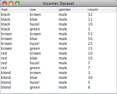
Again, like Gelman, I’m not convinced that Benford’s law can necessarily be used to draw conclusions on the presence or absence of vote tampering, but it is an interesting example of a Chi-square goodness-of-fit analysis, comparing some real-world data with a theoretical distribution, Benford’s law in this case. So I will demonstrate how to perform the analysis with Incanter using the data set made available by the Guardian. A CSV file with the data can be found here.
First load the necessary libraries,
(use '(incanter core stats charts io))and read the data using the read-dataset function.
(def votes (read-dataset "data/iran_election_2009.csv"
                         :header true))
Now, create variables representing the regions and the candidates.
(def regions (sel votes :cols "Region"))
(def ahmadinejad-votes (sel votes :cols "Ahmadinejad"))
(def mousavi-votes (sel votes :cols "Mousavi"))
(def rezai-votes (sel votes :cols "Rezai"))
(def karrubi-votes (sel votes :cols "Karrubi"))
We need to write a small function that will take a number and return only the first digit. We can do that by converting the number into a string with the str function, taking the first character of the string, and then converting that character into a number again.
(defn first-digit [x]
  (Character/digit (first (str x)) 10))
Now, map the first-digit function over the vote counts in each of the 30 regions for each candidate.
(def ahmadinejad (map first-digit ahmadinejad-votes))
(def mousavi (map first-digit mousavi-votes))
(def rezai (map first-digit rezai-votes))
(def karrubi (map first-digit karrubi-votes))
Now we have a list of first-digits across the different regions, for each candidate. Next, define function that implements Benford’s Law, create a variable containing the probabilities for each of the nine digits, and calculate the expected frequencies for the 30 regions.
(defn benford-law [d] (log10 (plus 1 (div d))))
(def benford-probs (benford-law (range 1 11)))
(def benford-freq (mult benford-probs (count regions)))
We will then need a function that takes the list of first digits for each candidate and returns the counts for each digit. We can use the :counts field returned by the tabulate function to do most of the work.
(defn get-counts [digits]
  (map #(get (:counts (tabulate digits)) % 0)
       (range 1.0 10.0 1.0)))
It’s always a good idea to look at the data, so plot the predicted first-digit frequencies and the frequencies for Ahmadinejad and Mousavi.
(doto (xy-plot (range 1 10) (get-counts ahmadinejad)
               :legend true :series-label "Ahmadinejad"
               :y-label "First digit frequency"
               :x-label "First digit"
               :title "First digit frequency by candidate")
      (add-lines (range 1 10) (get-counts mousavi)
                 :series-label "Mousavi")
      (add-lines (range 1 10) benford-freq
                 :series-label "Predicted")
      clear-background
      view)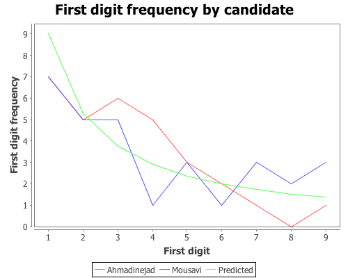
Based on that plot, the digit frequencies look like they follow Benford’s law. We can confirm that with a Chi-square goodness-of-fit test using the chisq-test function. Start with Ahmadinejad,
(def ahmadinejad-test
  (chisq-test :table (get-counts ahmadinejad)
              :probs benford-probs))
(:X-sq ahmadinejad-test)
(:p-value ahmadinejad-test)
The X-square test value is 5.439 with a p-value of 0.71. Based on these values we cannot reject the null hypothesis that the observed distribution of first-digits is the same as the expected distribution, which follows Benford’s law. Next test Mousavi’s vote counts,
(def mousavi-test
  (chisq-test :table (get-counts mousavi)
              :probs benford-probs))
(:X-sq mousavi-test)
(:p-value mousavi-test)
The X-square test value for Mousavi is 5.775 with a p-value of 0.672. Like Ahmadinejad, we cannot reject the null hypothesis. We might as well test the distributions of first-digits for the remaining two candidates (which we didn’t plot), Rezai and Karrubi.
(def rezai-test
  (chisq-test :table (get-counts rezai)
              :probs benford-probs))
(:X-sq rezai-test)
(:p-value rezai-test)
The X-square test value for Rezai is 12.834 with a p-value of 0.118, so we can’t reject the null hypothesis.
(def karrubi-test
  (chisq-test :table (get-counts karrubi)
              :probs benford-probs))
(:X-sq karrubi-test)
(:p-value karrubi-test)
Karrubi’s X-square value is 8.8696 with a p-value of 0.353, and like the other candidates appears to follow Benford’s law.
The conclusion based on the vote count summaries for the 30 Iranian regions, is that the votes follow Benford’s law.
Last-digit frequencies
Another approach to identifying vote tampering is to examine the last digit of the vote counts, instead of the first. This approach was discussed in this Washington Post article.
Unlike first-digits, last-digits don’t follow Benford’s law, but rather follow a uniform distribution. We can test the distribution of last-digits from our sample of 30 regions using the chisq-test function again. First, define a function to extract the last digit from a number,
(defn last-digit [x]
  (Character/digit (last (str x)) 10))
and map the function over the vote counts for each candidate.
(def ahmadinejad-last (map last-digit
                           ahmadinejad-votes))
(def mousavi-last (map last-digit
                       mousavi-votes))
(def rezai-last (map last-digit
                     rezai-votes))
(def karrubi-last (map last-digit
                       karrubi-votes))
Now we have a list of last-digits for the 30 regions for each candidate. We need to tweak the get-counts function, from above, so that it includes the digit zero, which wasn’t necessary in the first-digit case.
(defn get-counts [digits]
  (map #(get (:counts (tabulate digits)) % 0)
       (range 0.0 10.0 1.0)))
Now plot the last-digit distribution for each of hte candidates.
(doto (xy-plot (range 10)
               (get-counts ahmadinejad-last)
               :legend true
               :series-label "Ahmadinejad"
               :y-label "First digit frequency"
               :x-label "First digit"
               :title "Last digit frequency by candidate")
      (add-lines (range 10) (get-counts mousavi-last)
                 :series-label "Mousavi")
      (add-lines (range 10) (get-counts rezai-last)
                 :series-label "Rezai")
      (add-lines (range 10) (get-counts karrubi-last)
                 :series-label "Karrubi")
      clear-background
      view)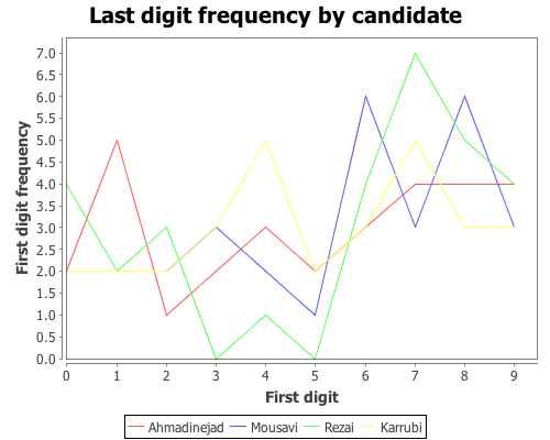
The data certainly doesn’t look like it’s following Benford’s law, but is it uniformly distributed? We can test that hypothesis with the chisq-test function, this time we won’t need to supply the :probs argument because a uniform distribution is the default.
(def ahmadinejad-test
  (chisq-test :table (get-counts ahmadinejad-last)))

(:X-sq ahmadinejad-test) ;; 4.667
(:p-value ahmadinejad-test) ;; 0.862

(def mousavi-test
  (chisq-test :table (get-counts mousavi-last)))
(:X-sq mousavi-test) ;; 8.667
(:p-value mousavi-test) ;; 0.469

(def rezai-test
  (chisq-test :table (get-counts rezai-last)))
(:X-sq rezai-test) ;; 15.333
(:p-value rezai-test) ;; 0.0822

(def karrubi-test
  (chisq-test :table (get-counts karrubi-last)))
(:X-sq karrubi-test) ;; 4.0
(:p-value karrubi-test) ;; 0.911
According to each of these tests, we cannot reject the hypothesis that the last-digits for each candidate follows a uniform distribution. The analysis written up in the Washington Post article came to the opposite conclusion, which is likely due to their use of more detailed data. The data used here was summary information for 30 regions. More detailed vote counts could certainly provide a different conclusion.
The complete code for this post can be found here.