Category Archives: Bayesian inference

The multinomial distribution is used to describe data where each observation is one of k possible outcomes. In his book, Bayesian Data Analysis (pg 83), Andrew Gelman demonstrates how to use Bayesian methods to make inferences about the parameters of a multinomial distribution. He used data from a sample survey by CBS news prior to the 1988 presidential election. In his book Bayesian Computation with R (pg. 60), Jim Albert used R to perform the same inferences on the same data as Gelman. I’ll now demonstrate how to perform these inferences in Clojure, with Incanter, using the sample-multinomial-params function. I will then describe the Bayesian model underlying sample-multinomial-params, and demonstrate how to do the same calculations directly with the sample-dirichlet function.

First, load the necessary libraries, including the incanter.bayes library.

(use '(incanter core stats bayes charts))

The data consist of 1447 survey responses; 727 respondents supported George Bush Sr., 583 supported Michael Dukakis, and 137 supported another candidate, or were undecided. Define a vector, y, that includes the counts for each of the outcomes.

(def y [727 583 137])

The proportion of supporters for the candidates, calculated by dividing y by the total responses,

(div y 1447)

are (0.502 0.403 0.095). If the survey data follows a multinomial distribution, these proportions are the parameters of that distribution. The question is, how good an estimate of the population parameters are these values?

Confidence intervals for the parameters can be calculated by applying the quantile function to a sample drawn from an appropriate distribution, which in the case of the parameters of a multinomial distribution is a Dirichlet distribution.

Samples can be drawn from the appropriate Dirichlet distribution with the sample-multinomial-params function.

(def  theta (sample-multinomial-params 1000 y))

This returns 1000 samples of the multinomial parameters, or probabilities of each of the outcomes in the data. Now, create variables representing the samples for each parameter,

(def theta1 (sel theta :cols 0))
(def theta2 (sel theta :cols 1))
(def theta3 (sel theta :cols 2))

and calculate the mean, standard deviation, 95% confidence interval, and display a histogram for each sample.

(mean theta1)
(sd theta1)
(quantile theta1 :probs [0.025 0.975]) 
(view (histogram theta1
                 :title "Bush, Sr. Support"))

The mean for theta1 is 0.502, the standard deviation is 0.013, and the 95% confidence interval is (0.476 0.528).

(mean theta2) 
(sd theta2)
(quantile theta2 :probs [0.025 0.975]) 
(view (histogram theta2
                 :title "Dukakis Support"))

The mean for theta2 is 0.403, the standard deviation is 0.013, and the 95% confidence interval is (0.376 0.427).

(mean theta3) 
(sd theta3)
(quantile theta3 :probs [0.025 0.975]) 
(view (histogram theta3
                 :title "Other/Undecided"))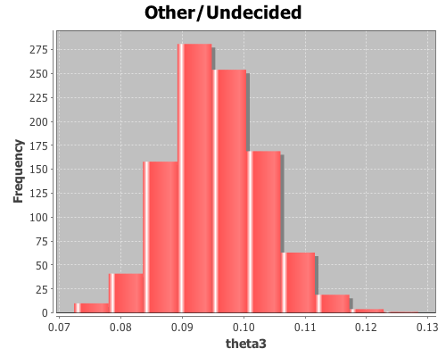

The mean for theta3 is 0.095, the standard deviation is 0.008, and the 95% confidence interval is (0.082 0.111).

Using the sample distributions for the parameters, we can view the distribution of other statistics, like the difference in support between Bush, Sr. and Dukakis. View a histogram of the difference in support for the two candidates.

(view (histogram (minus theta1 theta2) 
                 :title "Bush, Sr. and Dukakis Diff"))

The sample-multinomial-params functions returns values from a Dirichlet distribution. The Dirichlet is the conjugate prior distribution for the parameters of the multinomial distribution, such that the posterior Dirichlet’s parameters equal the sum of the count data, y, and the parameters from the prior Dirichlet, alpha.

Where

are the count data that follow a multinomial distribution,

are the parameters of the multinomial distribution, and

are the hyper-parameters of the prior Dirichlet distribution. The likelihood function, p(y | theta), is a multinomial conditional distribution that describes the likelihood of seeing the observed y values, given the values of the parameter, theta.

The prior, p(alpha), is made uninformative by setting all the alpha values equal to one, producing a uniform distribution.

Then the posterior Dirichlet becomes

Sample the proportions directly from the above Dirichlet distribution using the sample-dirichlet function.

(def alpha [1 1 1])
(def  props (sample-dirichlet 1000 (plus y alpha)))

This returns data from the same distribution as the sample-multinomial-params function, so all the means, standard deviations, and confidence intervals can be calculated as above.

The complete code for this example is here.