Linear regression with higher-order terms

This example will use a data set from NIST. It doesn’t represent the typical data used in regression, but it will provide an opportunity to perform regression with higher-order terms using Incanter.

You will need the incanter.core, incanter.stats, incanter.charts, and incanter.datasets libraries.

Load the necessary Incanter libraries.

(use '(incanter core stats charts datasets))

For more information on using these packages, see the matrices, datasets, and sample plots pages on the Incanter wiki.

Now load the NIST data set called filip, (you can find more information on this data set at http://www.itl.nist.gov/div898/strd/lls/data/Filip.shtml)

(def data (to-matrix (get-dataset :filip)))

Extract the y values,

(def y (sel data :cols 0))

and then use the sweep function to center the x values, in order to reduce collinearity among the polynomial terms

(def x (sweep (sel data :cols 1)))

Now take a look at the data:

(def plot (scatter-plot x y))
(view plot)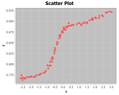

As you can see, this isn’t a typical data set, so we will use the same atypical model as NIST to fit the data:

y = b0 + b1*x + b2*x^2 + b3*x^3 + ... + b10*x^10

The following line of code creates a matrix of the polynomial terms x, x^2, x^3, x^4, x^5, x^6, x^7, x^8, x^9, x^10,

(def X (reduce bind-columns (for [i (range 1 11)] (pow x i))))

Run the regression, and view the results.

(def lm (linear-model y X))

Start with the overall model fit:

(:f-stat lm) ;; 2162.439
(:f-prob lm) ;; 1.1E-16

The model fits, now check out the R-square:

(:r-square lm) ;; 0.997

The model explains over 99% of the variance in the data. Like I said, not a typical data set.

View the estimates of the coefficients, and the p-values of their t-tests

(:coefs lm)
(:t-probs lm)

The values for coefficients b0, … b10 are (0.878 0.065 -0.066 -0.016 0.037 0.003 -0.009 -2.8273E-4 9.895E-4 1.050E-5 -4.029E-5), and the p-values are (0 0 0 1.28E-5 0 0.083 1.35E-12 0.379 3.74E-8 0.614 2.651E-5).

All the coefficients are significant except b5, b7, and b9.

Finally, overlay the fitted values on the original scatter-plot

(add-lines plot x (:fitted lm))

That’s the kind of fit rarely seen on real data! In fact, on real data this would be an example of over-fitting. This model likely wouldn’t generalize to new data from the same process that created this sample.

The complete code for this example is here.

Further Reading

• Linear regression (Wikipedia)