In addition to discovering Benford’s law (which I used in a previous post) 57 years before Frank Benford, Simon Newcomb made a series of measurements of the speed of light. In 1882 he measured the time in seconds that a light signal took to travel the 7,400 meters from the US Naval observatory, on the Potomac River, to a mirror at the base of the Washington Monument and back. Newcomb’s data are frequently used to demonstrate statistical techniques, as I will do here. The data are coded as deviations from 24,800 nanoseconds, so the first entry, corresponding to 24,828 nanoseconds, is 28.
Here’s a vector, x, containing the measurements.
(def x [28 -44 29 30 24 28 37 32 36
        27 26 28 29 26 27 22 23 20
        25 25 36 23 31 32 24 27 33
        16 24 29 36 21 28 26 27 27
        32 25 28 24 40 21 31 32 28
        26 30 27 26 24 32 29 34 -2
        25 19 36 29 30 22 28 33 39
        25 16 23])
There are two obvious outliers in the data, so the median, not the mean, is the preferred estimate of location. Bootstrapping is a method often employed for estimating confidence intervals, standard errors, and estimator bias for medians.
Load the necessary Incanter libraries,
(use '(incanter core stats charts))View a histogram of the data, note the two outlier observations at -2 and -44.
(view (histogram x
                 :nbins 20
                 :title "Newcomb's speed of light data"))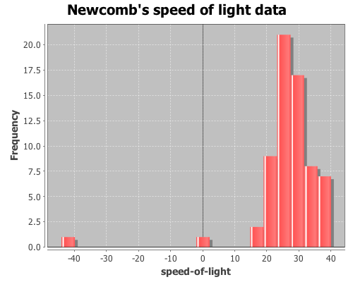
Now calculate the median of the sample data
(median x)The result is 27, but how does this value relate to the speed of light? We can translate this value to a speed in meters/sec with the following function.
(defn to-speed
  "Converts Newcomb's data into speed (meters/sec)"
  ([x] (div 7400 (div (plus 24800 x) 1E9))))
Now apply it to the median.
(to-speed (median x))The result is 2.981E8 m/sec (the true speed-of-light is now considered 2.9799E8 m/sec), but how good of an estimate of the median is this? How much sampling error is there? We can estimate confidence intervals, standard errors and estimator bias using bootstrapping.
Bootstrapping is a technique where items are drawn from a sample, with replacement, until we have a new sample that is the same size as the original. Since each item is replaced before the next item is drawn, a single value may appear more than once, and other items may never appear at all. The desired statistic, in this case median, is calculated on the new sample and saved. This process is repeated until you have the desired number of sample statistics. Incanter’s bootstrap function can be used to perform this procedure.
Draw 10,000 bootstrapped samples of the median.
(def t* (bootstrap x median :size 10000))View a histogram of the bootstrap sample of the median
(view (histogram t*
                 :density true
                 :nbins 20
                 :title "Bootstrap sample of medians"
                 :x-label "median"))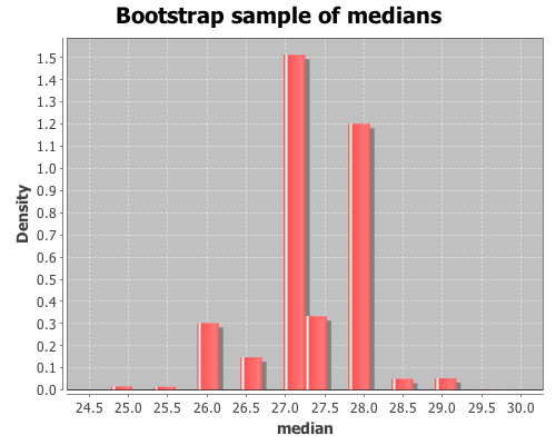
The bootstrap distribution is very jagged because the median is discrete, so there are only a small number of values that it can take. Later, I will demonstrate how to smooth over the discreteness of the median with the :smooth option to the bootstrap function.
The mean of t* is the bootstrap estimate of the median,
(mean t*)which is 27.301. An estimate of the 95% confidence interval (CI) for the median can be calculated with the quantile function.
(quantile t* :probs [0.025 0.975])The CI is estimated as (26.0 28.5). The standard error of the median statistic is estimated by the standard deviation of the bootstrap sample.
(sd t*)The standard error estimate is 0.681. The bias of the median statistic is estimated as the difference between it and the mean of the bootstrap sample.
(- (mean t*) (median x))The estimator bias is -0.3.
Smoothing
As was apparent in the previous histogram, the bootstrap distribution is jagged because the median is discrete. In order to smooth over the discreteness of the median, we can add a small amount of random noise to each bootstrap sample. The :smooth option adds gaussian noise to each median in the sample. The mean of the noise equals zero and the standard deviation equals 1/sqrt(n), where n is the original sample size.
Draw 10000 smoothed bootstrap samples of the median
(def smooth-t* (bootstrap x median
                          :size 10000
                          :smooth true))
View a histogram of the smoothed bootstrap samples of the median
(view (histogram smooth-t*
                 :density true
                 :nbins 20
                 :title "Smoothed bootstrap sample of medians"
                 :x-label "median"))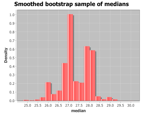
Calculate the estimate of the median.
(mean smooth-t*)The smoothed estimate of the median is 27.304. Now, calculate a 95% CI.
(quantile smooth-t* :probs [0.025 0.975])The smoothed result is (25.905 28.446).
The complete code for this example can be found here.