I want to discuss plans for future Incanter development, and I’m looking for volunteers interested in contributing to any of the following projects, as well as suggestions for other improvements.
My list of priorities, in no particular order:
1. Create new functions based on the Java libraries already included in Incanter. For instance, I would like to improve incanter.optimize by a) including the nonlinear optimization routines available in Parallel Colt b) writing new routines in Clojure, and c) improving the existing routines.
2. Integrate Parallel Colt’s sparse matrix support, as suggested by Mark Reid.
3. Expose more of the chart customizability of JFreeChart in the incanter.chart library, e.g. enabling annotations of categorical charts, allowing users to set the scale on axes, customizing colors, etc..
4. Create an incanter.viz library, consisting of Processing-based data visualizations.
7. Optimize existing functions; in general, I have favored ease-of-use and expressibility over performance, but there is A LOT of room to optimize without compromising usability.
Any other suggestions or feedback is welcome, and should be directed to the Incanter Goolge Group, where I have started an “Incanter Roadmap” thread. You can subscribe to the mailing list here.
The number of questions and suggestions I have been receiving about Incanter has been on the rise, so I decided to create a Google group (http://groups.google.com/group/incanter) as a central location for future discussion. To subscribe to the mailing list visit http://groups.google.com/group/incanter/subscribe. I welcome questions, answers, and suggestions for future development.
I would also like to thank everybody who has previously sent encouragement, patches, and improvements, it has made this project even more fun to work on.
The Processing language, created by Ben Fry and Casey Reas, “is an open source programming language and environment for people who want to program images, animation, and interactions.”
Incanter now includes the incanter.processing library, a fork of Roland Sadowski‘s clj-processing library, making it possible to create Processing visualizations with Clojure and Incanter. Incanter.processing provides much more flexibility when creating customized data visualizations than incanter.charts — of course, it is also more complex to use.
The processing website has a set of tutorials, including one on getting started, and there are also three great books on Processing worth checking out:
The API documentation for incanter.processing is still a bit underdeveloped, but is perhaps adequate when combined with the excellent API reference on the Processing website.
Incanter.processing was forked from of Roland Sadowski’s clj-processing library in order to provide cleaner integration with Incanter. I have added a few functions, eliminated some, and changed the names of others. There were a few instances where I merged multiple functions (e.g. *-float, *-int) into a single one to more closely mimic the original Processing API; I incorporated a couple functions into Incanter’s existing multi-methods (e.g. save and view); I eliminated a few functions that duplicated existing Incanter functions and caused naming conflicts (e.g. sin, cos, tan, asin, acos, atan, etc); and I changed the function signatures of pretty much every function in clj-processing to require the explicit passing of the ‘sketch’ (PApplet) object, whereas the original library passes it implicitly by requiring that it is bound to a variable called *applet* in each method of the PApplet proxy.
These changes make it easier to use Processing within Incanter, but if you just want to write Processing applications in Clojure without all the dependencies of Incanter, then the original clj-processing library is the best choice.
A Simple Example
The following is sort of a “hello world” example that demonstrates the basics of creating an interactive Processing visualization (a.k.a sketch), including defining the sketch’ssetup, draw, and mouseMoved methods and representing state in the sketch using closures and refs. This example is based on this one, found at John Resig‘s Processing-js website.
Click on the image above to see the live Processing-js version of the sketch.
Now define some refs that will represent the state of the sketch object,
(let [radius (ref 50.0)
      X (ref nil)
      Y (ref nil)
      nX (ref nil)
      nY (ref nil)
      delay 16
The variable radius will provide the value of the circle’s radius; X and Y will indicate the location of the circle; and nX and nY will indicate the location of the mouse. We use refs for these values because their values are mutable and need to be available across multiple functions in the sketch object.
Now define a sketch object, which is just a proxied processing.core.PApplet, and its required setup method,
sktch (sketch
        (setup []
          (doto this
            (size 200 200)
            (stroke-weight 10)
            (framerate 15)
            smooth)
          (dosync
            (ref-set X (/ (width this) 2))
            (ref-set Y (/ (width this) 2))
            (ref-set nX @X)
            (ref-set nY @Y)))
The first part of the setup method sets the size of the sketch, the stroke weight to be used when drawing, the framerate of the animation, and indicates that anti-aliasing should be used. The next part of the method uses a dosync block and ref-set to set initial values for the refs. Note the @ syntax to dereference (access the values of) the refs X and Y.
Processing sketches that use animation require the definition of a draw method, which in this case will be invoked 15 times per second as specified by the framerate.
The first part of the draw method uses dosync and ref-set to set new values for the radius, X, and Y refs for each frame of the animation. The sin function is used to grow and shrink the radius over time. The location of the circle, as indicated by X and Y, is determined by the mouse location (nX and nY) with a delay factor.
The next part of the draw method draws the background (i.e. gray background) and the circle with the ellipse function.
Finally, we need to define the mouseMoved method in order to track the mouse location, using the mouse-x and mouse-y functions, and set the values of the nX and nY refs. All event functions in incanter.processing, including mouseMoved, require an event argument; this is due to limitations of Clojure’s proxy macro, and isn’t required when using the Processing’s Java API directly.
Now that the sketch is fully defined, use the view function to display it,
(view sktch :size [200 200]))
The complete code for this example can be found here.
In future posts I will walk through other examples of Processing visualizations, some of which can be found in the Incanter distribution under incanter/examples/processing.
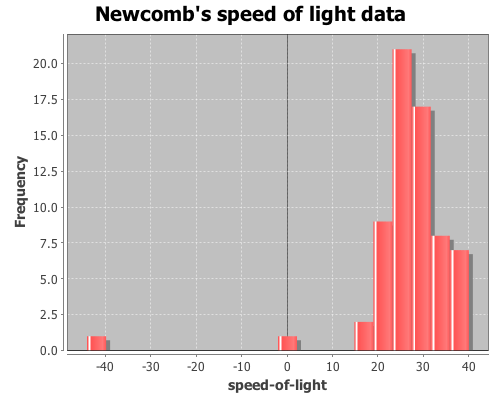
In addition to discovering Benford’s law (which I used in a previous post) 57 years before Frank Benford, Simon Newcomb made a series of measurements of the speed of light. In 1882 he measured the time in seconds that a light signal took to travel the 7,400 meters from the US Naval observatory, on the Potomac River, to a mirror at the base of the Washington Monument and back. Newcomb’s data are frequently used to demonstrate statistical techniques, as I will do here. The data are coded as deviations from 24,800 nanoseconds, so the first entry, corresponding to 24,828 nanoseconds, is 28.
View a histogram of the data, note the two outlier observations at -2 and -44.
(view (histogram x
                 :nbins 20
                 :title "Newcomb's speed of light data"))
Now calculate the median of the sample data
(median x)
The result is 27, but how does this value relate to the speed of light? We can translate this value to a speed in meters/sec with the following function.
(defn to-speed
  "Converts Newcomb's data into speed (meters/sec)"
  ([x] (div 7400 (div (plus 24800 x) 1E9))))
Now apply it to the median.
(to-speed (median x))
The result is 2.981E8 m/sec (the true speed-of-light is now considered 2.9799E8 m/sec), but how good of an estimate of the median is this? How much sampling error is there? We can estimate confidence intervals, standard errors and estimator bias using bootstrapping.
Bootstrapping is a technique where items are drawn from a sample, with replacement, until we have a new sample that is the same size as the original. Since each item is replaced before the next item is drawn, a single value may appear more than once, and other items may never appear at all. The desired statistic, in this case median, is calculated on the new sample and saved. This process is repeated until you have the desired number of sample statistics. Incanter’s bootstrap function can be used to perform this procedure.
Draw 10,000 bootstrapped samples of the median.
(def t* (bootstrap x median :size 10000))
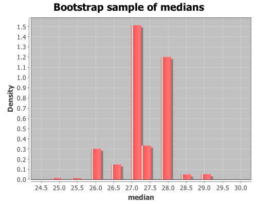
View a histogram of the bootstrap sample of the median
The bootstrap distribution is very jagged because the median is discrete, so there are only a small number of values that it can take. Later, I will demonstrate how to smooth over the discreteness of the median with the :smooth option to the bootstrap function.
The mean of t* is the bootstrap estimate of the median,
(mean t*)
which is 27.301. An estimate of the 95% confidence interval (CI) for the median can be calculated with the quantile function.
(quantile t* :probs [0.025 0.975])
The CI is estimated as (26.0 28.5). The standard error of the median statistic is estimated by the standard deviation of the bootstrap sample.
(sd t*)
The standard error estimate is 0.681. The bias of the median statistic is estimated as the difference between it and the mean of the bootstrap sample.
(- (mean t*) (median x))
The estimator bias is -0.3.
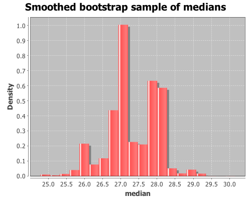
Smoothing
As was apparent in the previous histogram, the bootstrap distribution is jagged because the median is discrete. In order to smooth over the discreteness of the median, we can add a small amount of random noise to each bootstrap sample. The :smooth option adds gaussian noise to each median in the sample. The mean of the noise equals zero and the standard deviation equals 1/sqrt(n), where n is the original sample size.
Draw 10000 smoothed bootstrap samples of the median
(def smooth-t* (bootstrap x median
                          :size 10000
                          :smooth true))
View a histogram of the smoothed bootstrap samples of the median
The multinomial distribution is used to describe data where each observation is one of k possible outcomes. In his book, Bayesian Data Analysis (pg 83), Andrew Gelman demonstrates how to use Bayesian methods to make inferences about the parameters of a multinomial distribution. He used data from a sample survey by CBS news prior to the 1988 presidential election. In his book Bayesian Computation with R (pg. 60), Jim Albert used R to perform the same inferences on the same data as Gelman. I’ll now demonstrate how to perform these inferences in Clojure, with Incanter, using the sample-multinomial-params function. I will then describe the Bayesian model underlying sample-multinomial-params, and demonstrate how to do the same calculations directly with the sample-dirichlet function.
First, load the necessary libraries, including the incanter.bayes library.
(use '(incanter core stats bayes charts))
The data consist of 1447 survey responses; 727 respondents supported George Bush Sr., 583 supported Michael Dukakis, and 137 supported another candidate, or were undecided. Define a vector, y, that includes the counts for each of the outcomes.
(def y [727 583 137])
The proportion of supporters for the candidates, calculated by dividing y by the total responses,
(div y 1447)
are (0.502 0.403 0.095). If the survey data follows a multinomial distribution, these proportions are the parameters of that distribution. The question is, how good an estimate of the population parameters are these values?
Confidence intervals for the parameters can be calculated by applying the quantile function to a sample drawn from an appropriate distribution, which in the case of the parameters of a multinomial distribution is a Dirichlet distribution.
Samples can be drawn from the appropriate Dirichlet distribution with the sample-multinomial-params function.
(def theta (sample-multinomial-params 1000 y))
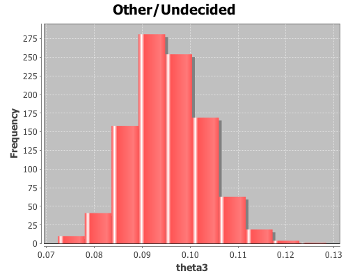
This returns 1000 samples of the multinomial parameters, or probabilities of each of the outcomes in the data. Now, create variables representing the samples for each parameter,
The mean for theta3 is 0.095, the standard deviation is 0.008, and the 95% confidence interval is (0.082 0.111).
Using the sample distributions for the parameters, we can view the distribution of other statistics, like the difference in support between Bush, Sr. and Dukakis. View a histogram of the difference in support for the two candidates.
The sample-multinomial-params functions returns values from a Dirichlet distribution. The Dirichlet is the conjugate prior distribution for the parameters of the multinomial distribution, such that the posterior Dirichlet’s parameters equal the sum of the count data, y, and the parameters from the prior Dirichlet, alpha.
Where
are the count data that follow a multinomial distribution,
are the parameters of the multinomial distribution, and
are the hyper-parameters of the prior Dirichlet distribution. The likelihood function, p(y | theta), is a multinomial conditional distribution that describes the likelihood of seeing the observed y values, given the values of the parameter, theta.
This returns data from the same distribution as the sample-multinomial-params function, so all the means, standard deviations, and confidence intervals can be calculated as above.
The basic premise is that you must choose one of three doors, one of which contains a prize. Once you have selected a door, Monty Hall reveals the contents of one of the doors you did not select, usually containing something like a goat. He then asks if you would like to switch your choice to the remaining unopened door. The question is, will switching doors increase you chances of winning, decrease your chances, or have no effect at all?
One thing to keep in mind, is that when Monty Hall shows you what’s behind one of the doors you didn’t select, he doesn’t ever reveal the door containing the prize. This fact should change your decision making process.
We can answer the question of which strategy is best by calculating the conditional probabilities of winning given you either switch or stay by performing a Monte Carlo simulation. The conditional probability of winning given you decide to switch doors can be written as Prob(win | switch), and is equal to the probability that you switch and win divided by the probability that you switch,
and the conditional probability of winning given you decide to stay with your original door is equal to the probability you stay and win divided by the probability that you stay.
Prob(win | stay) = Prob(stay & win)/Prob(stay)
In this simulation, we will generate a bunch of initial guesses, a bunch of prize locations, and a bunch of switch decisions and then use them to calculate the probabilities. First, load the necessary libraries.
(use '(incanter core stats charts))
Set a simulation sample size, generate samples of initial-guesses, prize-doors, and switch decisions with the sample function. The probability that the prize is behind any of the three doors is 1/3, as is the probability that you select a particular door as an initial guess, while the probability that you switch doors is 1/2.
Calculate the joint probability of winning and switching, by mapping the switch-win? function over the generated data, summing the occurrences of winning after switching, and then dividing this number by the total number of samples, n.
Calculate the probability of switching doors. Use the indicator and sum functions to calculate the frequency of switches, and then divide by the total number of samples.
Now repeat the process to calculate the conditional probability of winning given the decision to stay with your original choice. First, define a function that returns a one if a stay decision results in winning, zero otherwise.
The conditional probability of winning given you switch doors is approximately 0.66, while the probability of winning given you stay with your original choice is approximately 0.33.
To some this outcome may seem non-intuitive. Here’s why it’s the case: the probability that the prize is behind any of the three doors is 1/3, so once you have selected a door, the probability that the prize is behind a door you didn’t select is 2/3. Since Monty Hall knows which door has the prize, and never selects it as the door to reveal, all of the 2/3 probability belongs to the other unselected door. So switching will give you a 2/3 probability of winning the prize, and sticking with your original decision only gives you the original 1/3 chance.
The complete code for this example can be found here.
Benford’s law has been discussed as a means of analyzing the results of the 2009 Iranian election by several analysts. One of the first attempts was in a paper (pdf) by Boudewijn Roukema, where he concluded that the data did not follow Benford’s law, and that there was evidence for vote tampering. Andrew Gelman responded; he was not convinced by the statistics of this particular analysis (his criticism was of the statistical analysis, and didn’t reflect his opinion of the possibility of vote tampering).
Stochastic Democracy and the Daily Kos also used Benford’s law to analyze the election data, here, but came to the opposite conclusion of Roukema; the data did follow Benford’s law. A third analysis was performed by John Graham-Cumming in this blog post. He came to the same conclusion as Stochastic Democracy and Daily Kos, that the data did follow Benford’s law. His analysis is based on this data, available from the Guardian’s Data Blog.
Again, like Gelman, I’m not convinced that Benford’s law can necessarily be used to draw conclusions on the presence or absence of vote tampering, but it is an interesting example of a Chi-square goodness-of-fit analysis, comparing some real-world data with a theoretical distribution, Benford’s law in this case. So I will demonstrate how to perform the analysis with Incanter using the data set made available by the Guardian. A CSV file with the data can be found here.
First load the necessary libraries,
(use '(incanter core stats charts io))
and read the data using the read-dataset function.
We need to write a small function that will take a number and return only the first digit. We can do that by converting the number into a string with the str function, taking the first character of the string, and then converting that character into a number again.
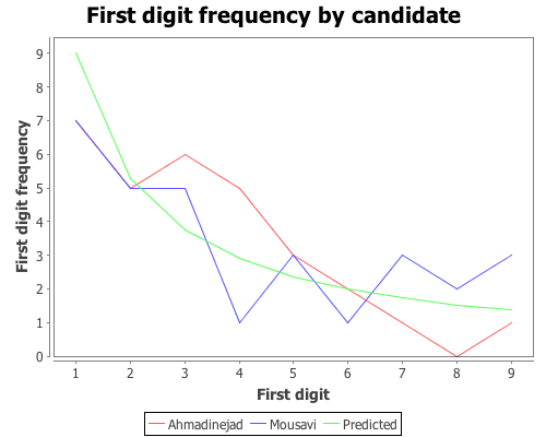
Now we have a list of first-digits across the different regions, for each candidate. Next, define function that implements Benford’s Law, create a variable containing the probabilities for each of the nine digits, and calculate the expected frequencies for the 30 regions.
We will then need a function that takes the list of first digits for each candidate and returns the counts for each digit. We can use the :counts field returned by the tabulate function to do most of the work.
Based on that plot, the digit frequencies look like they follow Benford’s law. We can confirm that with a Chi-square goodness-of-fit test using the chisq-test function. Start with Ahmadinejad,
The X-square test value is 5.439 with a p-value of 0.71. Based on these values we cannot reject the null hypothesis that the observed distribution of first-digits is the same as the expected distribution, which follows Benford’s law. Next test Mousavi’s vote counts,
The X-square test value for Mousavi is 5.775 with a p-value of 0.672. Like Ahmadinejad, we cannot reject the null hypothesis. We might as well test the distributions of first-digits for the remaining two candidates (which we didn’t plot), Rezai and Karrubi.
Karrubi’s X-square value is 8.8696 with a p-value of 0.353, and like the other candidates appears to follow Benford’s law.
The conclusion based on the vote count summaries for the 30 Iranian regions, is that the votes follow Benford’s law.
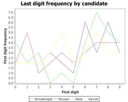
Last-digit frequencies
Another approach to identifying vote tampering is to examine the last digit of the vote counts, instead of the first. This approach was discussed in this Washington Post article.
Unlike first-digits, last-digits don’t follow Benford’s law, but rather follow a uniform distribution. We can test the distribution of last-digits from our sample of 30 regions using the chisq-test function again. First, define a function to extract the last digit from a number,
Now we have a list of last-digits for the 30 regions for each candidate. We need to tweak the get-counts function, from above, so that it includes the digit zero, which wasn’t necessary in the first-digit case.
The data certainly doesn’t look like it’s following Benford’s law, but is it uniformly distributed? We can test that hypothesis with the chisq-test function, this time we won’t need to supply the :probs argument because a uniform distribution is the default.
According to each of these tests, we cannot reject the hypothesis that the last-digits for each candidate follows a uniform distribution. The analysis written up in the Washington Post article came to the opposite conclusion, which is likely due to their use of more detailed data. The data used here was summary information for 30 regions. More detailed vote counts could certainly provide a different conclusion.
The complete code for this post can be found here.
We can use randomization (a.k.a. permutation tests) for significance testing by comparing a statistic calculated from a sample with the distribution of statistics calculated from samples where the null hypothesis is true.
In an earlier post, I demonstrated how to perform a t-test in Incanter. The p-value calculated for the test is based on the assumption that the distribution of test statistics when the null hypothesis, that the two sample means are identical, is true is a t-distribution. Let’s see if that assumption appears correct by generating 1000 samples of data where the null hypothesis is true, calculating the t-statistic for each, and then examining the distribution of statistics.
We can then compare the original t-statistic with this distribution and determine the probability of seeing that particular value when the null hypothesis is true. If the probability is below some cutoff (typically, 0.05) we reject the null hypothesis.
Start by loading the necessary libraries:
(use '(incanter core stats datasets charts))
Load the plant-growth data set.
(def data (to-matrix (get-dataset :plant-growth)))
Break the first column of the data into groups based on treatment type (second column) using the group-by function,
(def groups (group-by data 1 :cols 0))
The first group is the the control, the other two are treatments. View box-plots of the three groups, using the :group-by option of the box-plot function,
and view the test statistic and p-value for the first treatment,
(:t-stat t1)
(:p-value t1)
which are 1.191 and 0.2503, respectively, and the second treatment,
(:t-stat t2)
(:p-value t2)
which are -2.134 and 0.0479, respectively. These values provide evidence that the first treatment is not statistically significantly different from the control, but the second treatment is.
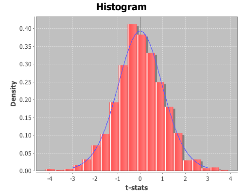
The above p-values are based on the assumption that the distribution of t-test statistics, when the null hypothesis is true, is a t-distribution. Let’s see if that assumption appears correct for these samples by generating 1000 samples where the null hypothesis is true. We can do that by permuting values between each of the treatments and the control using the sample-permutations function.
The distribution looks like a Student’s t. Now inspect the mean, standard deviation, and 95% confidence interval for the distribution from the first treatment.
(mean t-stats1)
The mean is 0.023,
(sd t-stats1)
the standard deviation is 1.064,
(quantile t-stats1 :probs [0.025 0.975])
and the 95% confidence interval is (-2.116 2.002). Since the t-statistics for the original sample, 1.191, falls within the range of the confidence interval, we cannot reject the null hypothesis; the mean of the first treatment and the control are statistically indistinguishable.
Now view their mean, sd, and 95% confidence interval for the second treatment,
(mean t-stats2)
The mean is -0.014,
(sd t-stats2)
The standard deviation is 1.054,
(quantile t-stats2 :probs [0.025 0.975])
and the 95% confidence interval is (-2.075 2.122). In this case, the original t-statistic, -2.134, is outside of the confidence interval, therefore the null hypothesis should be rejected; the second treatment is statistically significantly different than the control.
In both cases the permutation tests agreed with the standard t-test p-values. However, permutation tests can be used to test significance on sample statistics that do not have well known distributions like the t-distribution.
Comparing means without the t-statistic
Using a permutation test, we can compare means without using the t-statistic at all. First, define a function to calculate the difference in means between two sequences.
(defn means-diff [x y]
  (minus (mean x) (mean y)))
Calculate the difference in sample means between the first treatment and the control.
This returns 0.371. Now calculate the difference of means of the 1000 permuted samples by mapping the means-diff function over the rows returned by the sample-permutations function we ran earlier.
This returns a sequence of differences in the means of the two groups.
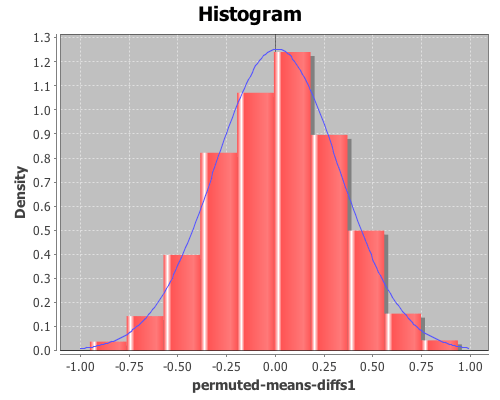
Plot a histogram of the perm-means-diffs1 using the density option, instead of the default frequency, and then add a pdf-normal curve with the mean and sd of perm-means-diffs data for a visual comparison.
The permuted data looks normal. Now calculate the proportion of values that are greater than the original sample means-difference. Use the indicator function to generate a sequence of ones and zeros, where one indicates a value of the perm-means-diff sequence is greater than the original sample mean, and zero indicates a value that is less.
Then take the mean of this sequence, which gives the proportion of times that a value from the permuted sequences are more extreme than the original sample mean (i.e. the p-value).
This returns 0.088, therefore the calculated p-value is 0.088, meaning that 8.8% of the permuted sequences had a difference in means at least as large as the difference in the original sample means. Therefore there is no evidence (at an alpha level of 0.05) that the means of the control and treatment-one are statistically significantly different.
We can also test the significance by computing a 95% confidence interval for the permuted differences. If the original sample means-difference is outside of this range, there is evidence that the two means are statistically significantly different.
(quantile perm-means-diffs1 :probs [0.025 0.975])
This returns (-0.606 0.595), but since the original sample mean difference was 0.371, which is inside the interval, this is further evidence that treatment one’s mean is not statistically significantly different than the control.
Now, calculate the p-values for the difference in means between the control and treatment two.
The calculated p-value is 0.022, meaning that only 2.2% of the permuted sequences had a difference in means at least as large as the difference in the original sample means. Therefore there is evidence (at an alpha level of 0.05) that the means of the control and treatment-two are statistically significantly different.
The original sample mean difference between the control and treatment two was -0.4939, which is outside the range (-0.478 0.466) calculated above. This is further evidence that treatment two’s mean is statistically significantly different than the control.
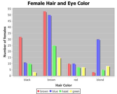
This example will demonstrate the use of the chisq-test function to perform tests of independence on a couple sample data sets.
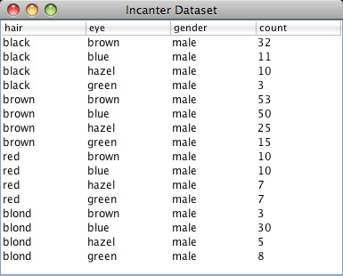
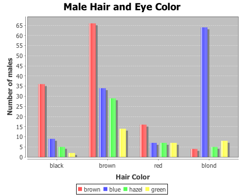
The first data set shows the number of male and female students with each of 16 different combinations of hair and eye color. We will use this data sample to test whether there is an association between hair and eye color. We will test males and females separately.
First load the necessary libraries.
(use '(incanter core stats charts datasets))
Now load the sample data with the get-dataset function, and then use group-by to break the data set into two groups based on gender (third column).
Both p-values are considerable below a 0.05 cut off threshold, indicating that the null hypothesis, that there is no association between eye and hair color, should be rejected for both males and females.
In addition to passing contingency tables as arguments to chisq-test, you can pass raw data using the :x and :y arguments, which we will do in the following example.
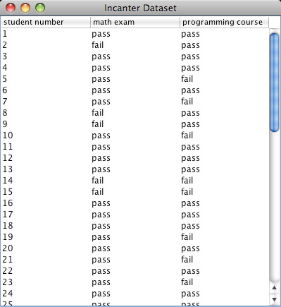
This example will test whether there is any correlation between the pass/fail results of a high school mathematics proficiency test and a freshman college programming course. The math-prog data set includes three columns: student_id, high school math proficiency test pass/fail results, and freshman college programming course pass/fail results.
First load the data, and convert the non-numeric data into integers with the to-matrix function.
In this case, we can’t reject null hypothesis, there is no association between the high school math proficiency exam and pass/fail rate of the freshman programming course.
The complete code for this example can be found here.
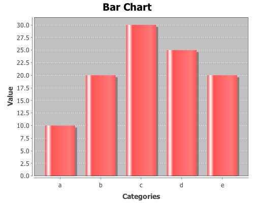
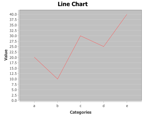
Yesterday, I received a question about plotting with non-numeric data. Unfortunately, the only way to do it in Incanter was to convert the data to numeric values, usually using the to-matrix function. So I have added two new functions, bar-chart and line-chart, that accept non-numeric data. In order to reduce the likelihood of confusing the line-plot function with the line-chart function, I renamed line-plot to xy-plot (which better reflects the name of the underlying JFreeChart class). The following are some examples of using these functions (for other plotting examples, see the sample plots and probability distributions pages of the Incanter wiki).
First, load the necessary libraries.
(use '(incanter core charts datasets))
Now plot a simple bar-chart. The first argument is a vector of categories, the second is a vector of values associated with each category.