
The multinomial distribution is used to describe data where each observation is one of k possible outcomes. In his book, Bayesian Data Analysis (pg 83), Andrew Gelman demonstrates how to use Bayesian methods to make inferences about the parameters of a multinomial distribution. He used data from a sample survey by CBS news prior to the 1988 presidential election. In his book Bayesian Computation with R (pg. 60), Jim Albert used R to perform the same inferences on the same data as Gelman. I’ll now demonstrate how to perform these inferences in Clojure, with Incanter, using the sample-multinomial-params function. I will then describe the Bayesian model underlying sample-multinomial-params, and demonstrate how to do the same calculations directly with the sample-dirichlet function.
First, load the necessary libraries, including the incanter.bayes library.
(use '(incanter core stats bayes charts))The data consist of 1447 survey responses; 727 respondents supported George Bush Sr., 583 supported Michael Dukakis, and 137 supported another candidate, or were undecided. Define a vector, y, that includes the counts for each of the outcomes.
(def y [727 583 137])The proportion of supporters for the candidates, calculated by dividing y by the total responses,
(div y 1447)are (0.502 0.403 0.095). If the survey data follows a multinomial distribution, these proportions are the parameters of that distribution. The question is, how good an estimate of the population parameters are these values?
Confidence intervals for the parameters can be calculated by applying the quantile function to a sample drawn from an appropriate distribution, which in the case of the parameters of a multinomial distribution is a Dirichlet distribution.
Samples can be drawn from the appropriate Dirichlet distribution with the sample-multinomial-params function.
(def theta (sample-multinomial-params 1000 y))
This returns 1000 samples of the multinomial parameters, or probabilities of each of the outcomes in the data. Now, create variables representing the samples for each parameter,
(def theta1 (sel theta :cols 0))
(def theta2 (sel theta :cols 1))
(def theta3 (sel theta :cols 2))
and calculate the mean, standard deviation, 95% confidence interval, and display a histogram for each sample.
(mean theta1)
(sd theta1)
(quantile theta1 :probs [0.025 0.975])
(view (histogram theta1
                 :title "Bush, Sr. Support"))
The mean for theta1 is 0.502, the standard deviation is 0.013, and the 95% confidence interval is (0.476 0.528).
(mean theta2)
(sd theta2)
(quantile theta2 :probs [0.025 0.975])
(view (histogram theta2
                 :title "Dukakis Support"))
The mean for theta2 is 0.403, the standard deviation is 0.013, and the 95% confidence interval is (0.376 0.427).
(mean theta3)
(sd theta3)
(quantile theta3 :probs [0.025 0.975])
(view (histogram theta3
                 :title "Other/Undecided"))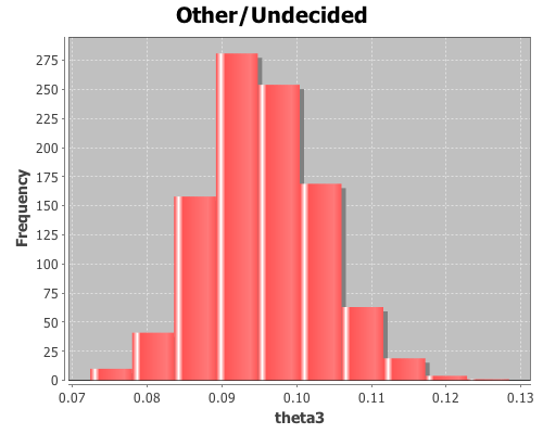
The mean for theta3 is 0.095, the standard deviation is 0.008, and the 95% confidence interval is (0.082 0.111).
Using the sample distributions for the parameters, we can view the distribution of other statistics, like the difference in support between Bush, Sr. and Dukakis. View a histogram of the difference in support for the two candidates.
(view (histogram (minus theta1 theta2)
                 :title "Bush, Sr. and Dukakis Diff"))
The sample-multinomial-params functions returns values from a Dirichlet distribution. The Dirichlet is the conjugate prior distribution for the parameters of the multinomial distribution, such that the posterior Dirichlet’s parameters equal the sum of the count data, y, and the parameters from the prior Dirichlet, alpha.

Where
are the count data that follow a multinomial distribution,

are the parameters of the multinomial distribution, and

are the hyper-parameters of the prior Dirichlet distribution. The likelihood function, p(y | theta), is a multinomial conditional distribution that describes the likelihood of seeing the observed y values, given the values of the parameter, theta.
The prior, p(alpha), is made uninformative by setting all the alpha values equal to one, producing a uniform distribution.
Then the posterior Dirichlet becomes

Sample the proportions directly from the above Dirichlet distribution using the sample-dirichlet function.
(def alpha [1 1 1])
(def  props (sample-dirichlet 1000 (plus y alpha)))
This returns data from the same distribution as the sample-multinomial-params function, so all the means, standard deviations, and confidence intervals can be calculated as above.
The complete code for this example is here.

Suppose, I have a matrix of Genetic data where each column is made of of Gene1 to Gene 23,000 say and say we have 6 columns. And in each each in each column, we have count data. Any idea how I should model this?
It sounds like you are working with either microarray expression data or possibly RNASeq data. If you want to perform statistical tests of any inferences you make, a sample size of six is very small!
However, my approach to analyzing that data would depend on what question I’m trying to answer.
Are you trying to estimate expression levels for each gene? Are you trying to detect differential expression across the six samples? Are you trying to identify clusters of genes that are active/inactive together in the different samples?
Mark Reimers at the National Cancer Institute wrote a nice guide to microarray data analysis called “An (Opinionated) Guide to Microarray Data Analysis”: http://discover.nci.nih.gov/microarrayAnalysis/Microarray.Home.jsp
That might give you some ideas on how to approach your analysis.
So far, the idea is just to madel the data using some Bayesian Method
Ah, if you want to use a Bayesian method to model the data, check out BEAM (Bayesian Estimation of Array Measurements).
Here’ the original paper:
Click to access denoising_recomb.pdf
And here’s the BEAM website, which as links to a web-based version of the program so you can upload your data directly and have it return the results.
http://people.csail.mit.edu/rondror/BEAM/
Was wondering how you could determine the minimum sample size required for the above example (i.e. the minimum amount of data needed for accurate prediction). Have read some papers on this, but am unsure how you would implement in R or Clojure. Thanks
Dave,
That is a great question, and one I should write an entire post about.
In the meantime, the only thing I can offer is yet another paper. The whitepaper, “Sample Size Determination for Multinomial Population” (pdf) by Subinoy Chakravarty is a nice summary of an approach with the associated references.
Even better, it has a nice table (table 1 on pg 2) for finding the sample size (n) for a given significance-level (alpha) and half-width of the confidence interval around the estimated proportions (d). For instance, to estimate the proportion parameters of a multinomial distribution within +/- 0.02 at a significance-level of 0.05, the minimum sample size, based on table 1, would be 3184.
I hope to create some power calculation functions for Incanter, and then write some posts on them, in the future.
David
Thanks for the quick response. Yes, am familiar with that paper and it hits the nail on the head of what I am trying to do, just not how I want to do it. Want to use Bayesian techniques (should have made that clear in my post) to come up with a sample size determination which is what led me to your post. Believe what you are doing above is a starting point, just not sure how to take it to the next level. Have read some papers on estimating multinomial params using Bayes (usually Dirichlet), just looking for a solid example/implementation to fill in the gaps for me. Thanks.
An alternative approach is to perform multiple simulations with different sample sizes (e.g. n1, n2, …) using the sample-multinomial-params function.
(def counts1 (mult n1 [p1 p2 p3]))
(def counts2 (mult n2 [p1 p2 p3]))
…
where p1, p2, p3 are the proportion parameters of your simulated multinomial distribution.
Now generate a sample of 1000 multinomial-parameters based on each of the different values of n:
(def params1 (sample-multinomial-params 1000 counts1))
(def params2 (sample-multinomial-params 1000 counts2))
Finally, plot the histograms for the simulated parameters and use the quantile function (just like in this post) to find the simulated-sample based on the smallest n with an acceptable confidence interval.
David
This approach does not seem to take into account the previous results. I.e, I start off and guess my initial params and simulate. I should then simulate again using updated params from the simulation I just ran. Somehow during all of this, I must also vary n. Just not sure how to approach from a purely Bayesian standpoint. Thanks for any/all help.
Alright, so would like some feedback on an approach to this. What I propose is more incremental and Bayesian in nature. Assume you only have 3 categories and start off with prior dirichlet params of 1,1,1 (similar to the last part of above). You then wait until you have data represented in all 3 categories (lets say this is n=10 and is distributed as 4,3,3). You then calculate the posterior as above (def props (sample-dirichlet 1000 (plus y alpha))with y=(4,3,3) and alpha=(1,1,1). You can then calculate means, sd, and CI for each param. If CI is within a given threshold, you are done (n is the sample size). If not, you increment n and take your next sample. You use the calculated means as your new dirichlet params and recalculate the posterior with updated y (i.e. 5,3,3). Does this at all make sense? Thanks
That should work, although I’m not sure you gain much by using the estimated means from the previous iteration, they should be stationary.
May have not explained well because the previous iteration provides update info for the next iteration. Assume three categories and we start with 4 in cat1, 3 in cat2, and 3 in cat3 (y=(4,3,3)). We assume we know nothing about the distro so we set alpha=(1,1,1). We generate 10k dirichlet and calc the means (.38, .31, .31). We now use these numbers as alpha and collect another sample such that y=(4,4,3). We generate 10k dirichlet again with updated y and alpha and get new means (.36,.36,.28). We now use these means as alpha and collect another sample such that y=(5,4,3). All the while, we are checking simultaneous confidence intervals for each multinomial param. When they are all within some certainty threshold, we stop and look at how many samples we have collected. This is our minimum sample size. May be missing the boat here, but this is my interpretation of bayesian updating. Let me know if I am way off course here.
I like it, seems like a reasonable approach.