Incanter 1.5.0 has been released!

After long development, the new version of Incanter has been released to clojars. This version contains a lot of changes, including following:

  • For matrix operations the clatrix/jblas libraries are used – this should greatly improve performance (but you may need to install libgfortran3 package on Linux 64-bit. See jblas wiki for more information)
  • Interpolation functions were added to incanter-core module
  • You can save charts in SVG format by using the new incanter-svg module
  • The incanter-chart module was extended with support for scatter plots
  • Many bugfixes

Full list of changes could be found in changelog. There are 2 open issues that could affect your use of Incanter, please read about them in changelog. We’ll try to address them in the next release.

I want to say “Thank You!” to all people who provided new functionality, fixed the bugs, filed the issues, and participated in discussions in mailing list. Without you, this release simply didn’t happen!

The next steps in development will happen in direction of release 2.0, where the main change will be use of core.matrix library for all matrix operations.

Hammock Driven Development Cheat Sheet

This last weekend I re-watched Rich Hickey’s excellent (I would say awesome, but he would disapprove) clojure-conj talk on Hammock Driven Development, which I’ve summarized into this one page cheat sheet. The talk isn’t specific to Clojure, and the ideas can, and have, been applied to domains outside of programming. I recommend it for anybody working on solving novel problems in any domain.

An Illustrated guide to multi-core parallelism in Clojure

Here are my Clojure Conj slides, From Concurrency to Parallelism: an illustrated guide to multi-core parallelism in Clojure. The version of clojure.par I used isn’t publicly available yet, but I will be publishing it in my github repo (github.com/liebke/clojure) soon, and hopefully it will make its way to master in the not too distant future.

I just want to thank everybody at the Conj for making it such a spectacular event! I’m already looking forward to next year.

Incanter executables

For a long time I’ve wanted a simple, double-clickable executable for Incanter, and now thanks to Alan Dipert’s swingrepl library I have it.

I have made an executable jar file, called incanter.jar, that launches a swingrepl, that includes Incanter and all of its dependencies, when double-clicked or started with the following command

java -jar incanter.jar

Note: Make sure to save incanter.jar with the .jar extension to ensure it executes correctly.

I have also used Apple’s Jar Bundler and SkoobySoft’s DMG Packager to create a Mac OS X executable that’s downloadable as a dmg file, Incanter.dmg.

Finally, I used Launch4j to create the Windows executable file,
Incanter.exe.

To build incanter.jar from source, use script/package in the Incanter distribution on Github, or just use lein uberjar (lein will call the file incanter-standalone.jar, and will create a non-executable jar called incanter.jar).

Reading and writing Excel (xls) files with Incanter

I have just added David James Humphreys’ incanter-excel module to the Incanter distribution, providing basic capabilities for reading Microsoft Excel spreadsheets in as Incanter datasets and saving datasets back out as xls files.

I have posted a simple spreadsheet of Australian airline passenger data from the 1950s to the Incanter website for the following example. The read-xls function can read xls files given either a filename or URL, so you won’t need to download the file.

Start by loading the necessary libraries, including incanter.excel.

(use '(incanter core charts excel))

Next, we can use the with-data macro to bind a dataset converted from the above xls file, using the read-xls function, and then view it.

(with-data (read-xls "http://incanter.org/data/aus-airline-passengers.xls")
  (view $data)

The read-xls function takes an optional argument called :sheet that takes either the name or index of the worksheet from the xls file to read (in this case either “dataset” or 0) , it defaults to 0.

[NOTE: A current weakness of read-xls is that cells containing formulae, as opposed to actual data, are not imported (i.e. the cells remain empty).]

Finally, we’ll create a time-series plot of the data. However, the time-series-plot needs time in milliseconds, so we’ll first create a function that converts the date column from Java Date objects to milliseconds, and then view the plot.

  (let [to-millis (fn [dates] (map #(.getTime %) dates))] 
    (view (time-series-plot (to-millis ($ :date)) ($ :passengers)))))

Datasets can also be saved as Excel files using the save-xls function. The following example just reads in one of the sample datasets using incanter.datasets/get-dataset and then saves it as an xls file.

(save-xls (get-dataset :cars) "/tmp/cars.xls")

The incanter-excel module is now included in the Incanter distribution on Github, and is available as a separate dependency from the Clojars repository. The complete code from this example can be found here.

Infix mathematical notation in Incanter

I obviously love Clojure’s prefix notation, but there are times when it is more concise, and familiar, to represent mathematical formulae using infix notation, so I have integrated the infix portion of Jeffrey Bester’s Clojure math library into Incanter. There is now a formula macro called $= for evaluating infix mathematical formulas in incanter.core.

Here’s an example,

user> (use 'incanter.core)
nil
user> ($= 7 + 8 - 2 * 6 / 2)
9

Note that there must be spaces between values and operators.

Vectors can be used instead of scalars. For instance, to add 5 to each element of the vector [1 2 3],

user> ($= [1 2 3] + 5)
(6 7 8)

or perform element-by-element arithmetic on vectors and matrices.

user> ($= [1 2 3] + [4 5 6])
(5 7 9)

user> ($= [1 2 3] * [1 2 3])
(1 4 9)

user> ($= [1 2 3] / [1 2 3])
(1 1 1)

user> ($= (matrix [[1 2] [4 5]]) + 6)
[ 7.0000  8.0000
10.0000 11.0000]

user> ($= (trans [[1 2] [4 5]]) + 6)
[7.0000 10.0000
8.0000 11.0000]

Examples of exponents using the ** function.

user> ($= 8 ** 3)
512.0

user> ($= 8 ** 1/2)
2.8284271247461903

user> ($= 2 ** -2)
0.25

user> ($= [1 2 3] ** 2)
(1.0 4.0 9.0)

Parens can be used for grouping,

user> ($= 10 + 20 * (4 - 5) / 6)
20/3

user> ($= (10 + 20) * 4 - 5 / 6)
715/6

user> ($= 10 + 20 * (4 - 5 / 6))
220/3

including arbitrarily nested groupings.

user> ($= ((((5 + 4) * 5))))
45

Of course, variables can be used within the formula macro,

user> (let [x 10
            y -5]
        ($= x + y / -10))
21/2

and mathematical functions like sin, cos, tan, sq, sqrt, etc. can be used with standard Clojure prefix notation.

user> ($= (sqrt 5) * 5 + 3 * 3)
20.18033988749895

user> ($= sq [1 2 3] + [1 2 3])
(2 6 12)

user> ($= sin 2 * Math/PI * 2)
5.713284232087328

user> ($= (cos 0) * 10)
10.0

user> ($= (tan 2) * Math/PI * 10)
-68.64505182223235

user> ($= (asin 1/2) * 10)
5.23598775598299

user> ($= (acos 1/2) * 10)
10.47197551196598

user> ($= (atan 1/2) * 10)
4.636476090008061

Functions can also be applied to vectors,

user> ($= [1 2 3] / (sq [1 2 3]) + [5 6 7])
(6 13/2 22/3)

user> ($= [1 2 3] + (sin [4 5 6]))
(0.2431975046920718 1.0410757253368614 2.720584501801074)

Boolean tests are also supported.

user> ($= 3 > (5 * 2/7))
true

user> ($= 3 <= (5 * 2/7))
false

user> ($= 3 != (5 * 2/7))
true

user> ($= 3 == (5 * 2/7))
false

user> ($= 3 != 8 && 6 < 12)
true

user> ($= 3 != 8 || 6 > 12)
true

Matrix multiplication uses the <*> function (equivalent to R’s %*% operator).

user> ($= [1 2 3] <*> (trans [1 2 3]))
[1.0000 2.0000 3.0000
2.0000 4.0000 6.0000
3.0000 6.0000 9.0000]

user> ($= (trans [[1 2] [4 5]]) <*> (matrix [[1 2] [4 5]]))
[17.0000 22.0000
22.0000 29.0000]

user> ($= (trans [1 2 3 4]) <*> [1 2 3 4])
30.0

user> ($= [1 2 3 4] <*> (trans [1 2 3 4]))
[1.0000 2.0000  3.0000  4.0000
2.0000 4.0000  6.0000  8.0000
3.0000 6.0000  9.0000 12.0000
4.0000 8.0000 12.0000 16.0000]

The Kronecker product uses the <x> function (equivalent to R’s %x% operator).

user> ($= [1 2 3] <x> [1 2 3])
[1.0000
2.0000
3.0000
2.0000
4.0000
6.0000
3.0000
6.0000
9.0000]

user> ($= (matrix [[1 2] [3 4] [5 6]]) <x> 4)
[ 4.0000  8.0000
12.0000 16.0000
20.0000 24.0000]

user> ($= (matrix [[1 2] [3 4] [5 6]]) <x> (matrix [[1 2] [3 4]]))
[ 1.0000  2.0000  2.0000  4.0000
 3.0000  4.0000  6.0000  8.0000
 3.0000  6.0000  4.0000  8.0000
 9.0000 12.0000 12.0000 16.0000
 5.0000 10.0000  6.0000 12.0000
15.0000 20.0000 18.0000 24.0000]

user> ($= [1 2 3 4] <x> 4)
[ 4.0000
 8.0000
12.0000
16.0000]

user> ($= [1 2 3 4] <x> (trans [1 2 3 4]))
[1.0000 2.0000  3.0000  4.0000
2.0000 4.0000  6.0000  8.0000
3.0000 6.0000  9.0000 12.0000
4.0000 8.0000 12.0000 16.0000]

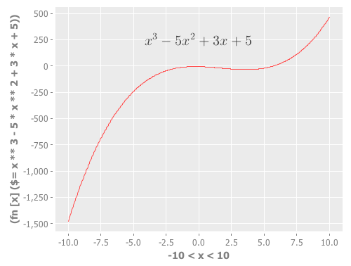
Here’s an example using the formula macro in a function-plot of x^3 - 5x^2 + 3x +5 , (I will use the incanter.latex/add-latex function to add a LaTeX annotation to the chart).

(use '(incanter core charts latex))
(doto (function-plot (fn [x] ($= x ** 3 - 5 * x ** 2 + 3 * x + 5)) -10 10)
  (add-latex 0 250 "x^3 - 5x^2 + 3x +5")
  view)

The next example will use the car-speed-to-breaking-distance sample data (the :cars dataset). I’ll partition the data, first selecting rows where the ratio of dist/speed is less than 2, then selecting rows where the ratio is greater than 2, and finally adding a line showing this threshold.

First, use the with-data macro, passing it the :cars sample data. Then apply the $where function in order to filter the data; pass it a $fn, which is a bit of syntax sugar around Clojure’s fn function that does map destructuring for functions that operate on dataset rows. For instance

($fn [x y] (…))

becomes

(fn [{:keys x y}] (…))

The parameter names specified in $fn must correspond to the column names of the dataset.

(use '(incanter core datasets charts))
(with-data (get-dataset :cars)
  (doto (scatter-plot :speed :dist 
          :data ($where ($fn [speed dist] 
                          ($= dist / speed < 2))))
    (add-points :speed :dist 
      :data ($where ($fn [speed dist] 
                      ($= dist / speed >= 2))))
    (add-lines ($ :speed) ($= 2 * ($ :speed)))
    view))

The complete code for this post is available here.

Adding LaTeX equations to Incanter charts

I’ve added a new library to Incanter called incanter.latex that adds the ability to include LaTeX formatted equations as annotations and subtitles in charts. The library is based on the fantastically useful JLaTeXMath library.

The following examples require Incanter version 1.2.2-SNAPSHOT or greater. Add the following dependency to your project.clj file:

[incanter "1.2.2-SNAPSHOT"]

Load the necessary libraries.

(use '(incanter core stats charts latex))

Define the latex-formatted equation; I’ll use the str function so I can break the equation across multiple lines. Notice that I have to use two backslashes where I would only need one if I were were working directly in LaTeX; this is because the backslash is an escape character in Clojure/Java strings.

(def eq (str "f(x)=\\frac{1}{\\sqrt{2\\pi \\sigma^2}}" 
             "e^{\\frac{-(x - \\mu)^2}{2 \\sigma^2}}"))

The equation can be rendered as an image with the latex function. The rendered equation can then be viewed in a window or saved as a png file with the view and save functions respectively.

(view (latex eq))
(save (latex eq) filename)

Use the add-latex function to add an annotation to a chart. The following example adds the above equation to a function-plot of the Normal PDF.

(doto (function-plot pdf-normal -3 3)
  (add-latex 0 0.1 eq)
  view)

Use the add-latex-subtitle function to add a rendered LaTeX equation as a subtitle to the chart (this particular chart does not have a main title).

(doto (function-plot pdf-normal -3 3)
  (add-latex-subtitle eq)
  view)

The complete code for the above examples can be found here.

New default theme and customization features for Incanter charts

I just updated Incanter‘s default chart theme. The new theme is inspired by Hadley Wickham‘s awesome ggplot2 package for R.

The first example is my usual “hello world” chart, a histogram of data sampled from a normal distribution.

(use '(incanter core charts stats datasets))

(view (histogram (sample-normal 1000)))

The next example is a scatter plot of the sepal-length vs. sepal-width from the built-in iris data set.

(view (scatter-plot :Sepal.Length :Sepal.Width :data (get-dataset :iris)))

In addition to changing the default theme, I have included new functions for customizing the appearance of the charts. Here’s an example of the set-stroke function, used here to change the color of the data points in the previous chart.

(doto (scatter-plot :Sepal.Length :Sepal.Width :data (get-dataset :iris))
  (set-stroke-color java.awt.Color/gray)
  view)

The next example uses the :group-by option to color the points based on their species.

(view (scatter-plot :Sepal.Length :Sepal.Width 
                    :group-by :Species 
                    :data (get-dataset :iris)))

This example uses function-plot to create an xy-plot of the sine and cosine functions.

(doto (function-plot sin -10 10)
  (add-function cos -10 10)
  view)

This example uses the $rollup and bar-chart functions to plot the data from the built-in hair-eye-color data set.

(with-data (->>  (get-dataset :hair-eye-color)
             ($rollup :sum :count [:hair :eye]))
  (view (bar-chart :hair :count :group-by :eye :legend true)))

This example uses the box-plot function to plot data from three gamma distributions.

(doto (box-plot (sample-gamma 1000 :shape 1 :rate 2)
                :legend true :y-label "")
  view 
  (add-box-plot (sample-gamma 1000 :shape 2 :rate 2))
  (add-box-plot (sample-gamma 1000 :shape 3 :rate 2)))

The following examples are based on the charts in figure 4.2 of chapter four of “The Joy of Clojure“, where the performance characteristics of Clojure’s data structures are discussed.

First define the two functions to plot, and the range of values to plot them over.

(defn log32 [x] (/ (log x) (log 32)))
(defn f1 [n] (plus (log2 n) (mult (log32 n) 5000)))
(defn f2 [n] n)

(def min-val 10)
(def max-val 40000)

Next, create the plot and use the set-stroke function to increase the stroke thickness for both lines, and make the second line dashed.

(def chart (doto (function-plot f1 min-val max-val 
                   :legend true 
                   :series-label "O(log2 n) + O(log32 n) * 5000"
                   :x-label ""
                   :y-label "")
             (add-function f2 min-val max-val 
                           :step-size 5000 
                           :series-label "O(n)") 
             (set-stroke :width 2)
             (set-stroke :width 2 :dataset 1 :dash 5)))

(view chart)

The three charts in the book are of the same data but each focuses on a different region. You can use the set-y-range and set-x-range functions to zoom-in on each of the different regions.

;; PLOT (A)
(doto chart
  (set-title "(A)")
  (set-x-range 100 5000)
  (set-y-range 30 12000))

;; PLOT (B)
(doto chart
  (set-title "(B)")
  (set-y-range 10000 16000)
  (set-x-range 10000 16000))

;; PLOT (C)
(doto chart
  (set-title "(C)")
  (set-y-range 0 30000)
  (set-x-range 0 30000))

The new theme is available in the latest version of Incanter on Clojars and Github, and the complete code for the above examples is available here.

Incanter has migrated to Leiningen

I have completed the process of migrating Incanter from the Maven build tool to Leiningen.

Incanter now includes several project.clj files, one for the overall project and one for each submodule. The top-level project.clj file builds what was formerly called incanter-app/incanter-full using the modules incanter-core, incanter-charts, incanter-processing, incanter-io, incanter-pdf, and incanter-mongodb.

The modules live in the modules/ directory, and each is an independent Leiningen project that can be built as a standalone library.

The script/ directory has repl and swank scripts (both sh and bat) stolen from labrepl, and simple scripts for managing the builds of all the modules (install, test, clean).

One bonus of this change is that I have been able to push Incanter and its modules back on to Clojars.org.

To include the full library as a dependency in your Leiningen project, add the following entry to your project.clj file:

[incanter "1.2.1-SNAPSHOT"]

If you only want to include a subset of Incanter’s functionality in your project, use one of the following modules instead:

 [incanter/incanter-core "1.2.1-SNAPSHOT"]
 [incanter/incanter-charts "1.2.1-SNAPSHOT"]
 [incanter/incanter-io "1.2.1-SNAPSHOT"]
 [incanter/incanter-processing "1.2.1-SNAPSHOT"]
 [incanter/incanter-pdf "1.2.1-SNAPSHOT"]
 [incanter/incanter-mongodb "1.2.1-SNAPSHOT"]

Updated build instructions can be found in the new README available in Incanter’s Github repository.

Dynamic data tables with Incanter

In a previous post, Dynamic charts with Incanter, I demonstrated how sliders can be linked to either an xy-plot or a scatter-plot. In this post I’ll demonstrate how sliders can be used to manipulate a dataset query, and dynamically update the results in a table.

Start by using the get-dataset function to load the iris sample data. Next, create a Swing JTable object containing the data with the data-table function, and then view it.

(use '(incanter core charts datasets))

(let [data (get-dataset :iris)
      table (data-table data)]
  (view table)

Use the sliders macro to create two sliders; one bound to species, a vector of iris species values, and the other bound to min-petal-length, a range of petal-lengths that will provide the lower bound for a query, and then create the expression that will be evaluated when the sliders are manipulated.

  (sliders [species ["setosa" "virginica" "versicolor"]
            min-petal-length (range 0 8 0.1)]
    (set-data table ($where {:Species species 
                             :Petal.Length {:gt min-petal-length}} 
                            data))))

In this case, the expression uses the set-data multi-method to update the values of the data-table with the results from a $where query.

Manipulating the sliders changes the query values, and dynamically updates the rows in the table.

Although it would be more natural to use a drop-down option menu, check-boxes, or radio-buttons to manipulate the species values, this example demonstrates that non-numeric values can be bound to sliders.

The data-table function and set-data multi-method are available in the latest version of Incanter on Github and on repo.incanter.org.