Category Archives: Clojure

FlightCaster merges its statistical-learning code into Incanter

Two goals have always been kept in mind during the development of Incanter 1) to provide an R-like, interactive statistical and graphics environment for performing data analysis, and 2) to provide a collection of libraries that can be embedded in larger data analysis systems, taking advantage of both the power of the Clojure language and the rich set of libraries available on the JVM for accessing and processing data.

Incanter has provided much of what you would expect from R by combining the power of the Clojure language with Java libraries, like Parallel Colt, jFreeChart, and Processing. The Clojure language itself is well suited for data processing due to its data structures, the sequence abstraction, the powerful sequence processing functions, destructuring, data structure literals, and myriad other niceties.

Now, Incanter’s goal of being embed-able in larger data analysis systems has taken a giant step forward with the merger of Flightcaster‘s code. Flightcaster’s service for predicting airline arrival times is a Clojure- and Hadoop-based distributed statistical-learning system that now has Incanter at the core. Their setup demonstrates how Incanter can scale up to larger data sets by leveraging JVM-based projects like Hadoop, AKKA, or other Clojure-based distributed computing systems. And with the Flightcaster code, Incanter has new functionality in classification, information theory, more probability, more io capabilities, a large range of dependence and similarity measures, and a variety of data transformation functions.

And this marks just the beginning of Flightcaster’s participation in the development of Incanter. Together we are working on a number of algorithms for learning models, structure, ensembles, and more. Future work will also ensure that Incanter can work seemlessly with FlightCaster’s recently open-source Crane framework for managing distributed processes on Hadoop and Amazon’s EC2.

Building a Clojure Web application with Incanter, Compojure, and Leiningen

This post will demonstrate how to build a simple Clojure Web application, with Compojure, that will use Incanter to generate a sample from a normal distribution with parameters (size, mean, and standard deviation) provided by the user, and then return a PNG image of the histogram of the data.

This example is simple, but it demonstrates how to dynamically generate an Incanter chart and pass it directly to the Web client as a PNG image.

For more information on the Compojure Web framework, visit its Github repository, its Google group, its WikiBooks site, and this quick tutorial.

I will use the Leiningen build tool to download dependencies, compile the application, and package it up as jar file. For more information on installing and using Leiningen, see my previous post.

Let’s start off by creating a project directory, I’ll call it incanter-webapp, and give it a src subdirectory. Then create the following Leiningen project.clj file in the project directory.

(defproject incanter-webapp "0.1.0"
  :description "A simple Incanter web-app."
  :dependencies [[incanter "1.2.1-SNAPSHOT"]
                 [compojure "0.3.2"]]
  :main simple_web_app)

This project file includes two dependencies, Incanter and Compojure, and indicates that the -main function for the project is in the file simple_web_app.clj in the src subdirectory of the project.

Next create the file called simple_web_app.clj in the src subdirectory.

(ns simple_web_app
  (:gen-class)
  (:use [compojure]
        [compojure.http response]
        [incanter core stats charts])
  (:import (java.io ByteArrayOutputStream
                    ByteArrayInputStream)))

Note that the namespace for this file is simple_web_app with underscores like in the file name and in the :main line of the project.clj file.

In Compojure, you need to define routes, which in this case associate the function sample-form with “/”, and the function gen-samp-hist-png with “/sample-normal”.

(defroutes webservice
  (GET "/"
    sample-form)
  (GET "/sample-normal"
    (gen-samp-hist-png request
                       (params :size)
                       (params :mean)
                       (params :sd))))

The function gen-samp-hist-png takes four arguments, a request object, the sample size, the population mean, and the population standard deviation, and then updates the Compojure response object to include an Incanter histogram of a sample from a normal distribution with the given parameters.

Now define the gen-samp-hist-png function; start by converting the string-arguments, passed in from the params object, into numbers.

(defn gen-samp-hist-png
  [request size-str mean-str sd-str]
    (let [size (if (nil? size-str)
                 1000
                 (Integer/parseInt size-str))
          m (if (nil? mean-str)
              0
              (Double/parseDouble mean-str))
          s (if (nil? sd-str)
              1
              (Double/parseDouble sd-str))

Each argument has a default value, 1000 for size, 0 for mean, and 1 for the standard deviation (sd).

Next generate the sample from the normal distribution using Incanter’s sample-normal function with the given size, mean, and standard deviation, and then create a histogram of the resulting data.

          samp (sample-normal size
                              :mean m
                              :sd s)
          chart (histogram
                  samp
                  :title "Normal Sample"
                  :x-label (str "sample-size = " size
                                ", mean = " m
                                ", sd = " s))

I’ve used the x-label option of the histogram function to customize the x-axis label so that it includes the given sample size, mean, and standard deviation.

Next, we need to convert the histogram into a byte array, and feed that into a ByteArrayInputStream that can be passed to Compojure’s update-response function, along with a header that sets the Content-Type to “image/png”.

        out-stream (ByteArrayOutputStream.)
        in-stream (do
                    (save chart out-stream)
                    (ByteArrayInputStream.
                      (.toByteArray out-stream)))
        header {:status 200
                :headers {"Content-Type" "image/png"}}]
    (update-response request
                     header
                     in-stream)))

The above code is the key to sending a dynamically generated chart directly to the client. In addition to a filename, an OutputStream can be passed to Incanter’s save function; in this case, we use a ByteArrayOutputStream, which is then converted to a byte array that is used to initialize the ByteArrayInputStream that is passed to update-response.

We can create a Web form for submitting requests to /sample-normal. The following function is a helper function that creates a simple html page skeleton.

(defn html-doc
  [title & body]
  (html
    (doctype :html4)
    [:html
      [:head
        [:title title]]
      [:body
       [:div
	[:h2
	 [:a {:href "/"}
          "Generate a normal sample"]]]
        body]]))

Now define the sample-form function, which will generate a Web form using html-doc. This function was associated with “/” earlier using the defroutes macro.

(def sample-form
  (html-doc "sample-normal histogram"
    (form-to [:get "/sample-normal"]
      "sample size: " (text-field {:size 4} :size)
      "mean: " (text-field {:size 4} :mean)
      "sd: " (text-field {:size 4} :sd)
      (submit-button "view"))))

Now, we need to create a -main function that will be called when the incanter-webapp.jar is executed. This function will call Compojure’s run-server function, starting the built-in Jetty server on port 8080.

(defn -main [& args]
  (run-server {:port 8080}
    "/*" (servlet webservice)))

Now we can use Leiningen to download and install all the necessary dependencies, including Incanter and Compojure, and then build and package the app.

$ lein deps
$ lein compile
$ lein uberjar

Finally, to start the server, run

$ java -jar incanter-webapp-standalone.jar 

and visit http://localhost:8080 to submit a request, or go directly to the sample-normal app by constructing a URL like the following:

http://localhost:8080/sample-normal?size=500&mean=100&sd=10

Which returns a PNG image of a histogram like this:

The complete code for this example can be found here, and the Leiningen project file can be found here.

Incanter Cheat Sheet

I’ve created an Incanter cheat sheet (pdf or LaTex) based on Steve Tayon’s Clojure cheat sheet (pdf or html). Click on the image below to see the complete pdf.

Updated: Trimmed some redundancies, got the sheet down to a single page.

Statistical Learning in Clojure Part 1: LDA & QDA Classifiers

This will hopefully be the first of a series of posts based on a book that has substantially influenced me over the last several years, The Elements of Statistical Learning (EoSL) by Hastie, Tibshirani, and Friedman (I went and got a degree in statistics essentially for the purposes of better understanding this book). Best of all, the pdf version of EoSL is now available free of charge at the book’s website, along with data, code, errata, and more.

This post will demonstrate the use of Linear Discriminant Analysis and Quadratric Discriminant Analysis for classification, as described in chapter 4, “Linear Methods for Classification”, of EoSL.

I will implement the classifiers in Clojure and Incanter, and use the same data set as EoSL to train and test them. The data has 11 different classes, each representing a vowel sound, and 10 predictors, each representing processed audio information captured from eight male and seven female speakers. Details of the data are available here. The data is partitioned into a training set and a test set.

The task is to classify each of the N observations as one of the (K=11) vowel sounds using the (p=10) predictors. I will do this using a Bayes classifier built from both linear- and quadratic-discriminant functions. The Bayes classifier works by estimating the probability that an observation, x, belongs to each class, k, and then selects the class with the highest probability. Appropriately, Bayes rule is used to calculate the conditional probability , or posterior probability, for each class.

(eq 4.7) P(G=k|X=x) = \frac{P(X=x|G=k)\pi_k}{\sum_{l=1}^{K} P(X=x|G=l)\pi_l}  

Where, \pi_k is the prior probability of class k. If we model each class density as multivariate-normal, then P(X=x|G=k) = f_k(x) , where

(eq 4.8) f_{k}(x) = \frac{1}{(2\pi)^{p/2}|\Sigma_k|^{1/2}}e^{-\frac{1}{2}(x-\mu_k)^T\Sigma_{k}^{-1}(x-\mu_k)}  

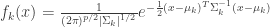
and the posterior probability becomes

(eq 4.7) P(G=k|X=x) = \frac{f_{k}(x)\pi_k}{\sum_{l=1}^{K}f_l(x)\pi_l}  

Since the denominator is the same for each class, we can ignore it, and if we take the log of the numerator and ignore the constant, (2\pi)^{p/2} , in the density function, we end up with the quadratic discriminant function:

(eq 4.12) \delta_{k}(x)=-\frac{1}{2}log|\Sigma_{k}|-\frac{1}{2}(x-\mu_k)^T\Sigma_{k}^{-1}(x-\mu_k)+log\pi_k 

If we further assume that the covariance matrices, \Sigma_k are equal for each cluster, then more terms cancel out and we end up with the linear discriminant function,

(eq 4.10) \delta_{k}(x)=x^T\Sigma^{-1}\mu_k-\frac{1}{2}\mu_k^T\Sigma^{-1}\mu_k+log\pi_k  

Classification is then performed with these discriminant functions using the following decision rule:

(eq 4.10a) G(x)=argmax_k\delta_k(x) 

In other words, select the class, k, with the highest score for each observation.

Implementing the LDA Classifier

Start by loading the necessary Incanter libraries and the data sets from the EoSL website:

(use '(incanter core stats charts io))
(def training (to-matrix 
                (read-dataset "http://bit.ly/464h4h" 
                              :header true)))
(def testing (to-matrix 
               (read-dataset "http://bit.ly/1btCei" 
                             :header true)))

Define the fixed parameters:

(def K 11)
(def p 10)
(def N (nrow training))
(def group-counts (map nrow (group-by training 1)))

Since we don’t know the parameters of the multivariate-normal distributions used to model each cluster, we need to estimate them with the training data. First, estimate the prior probabilities for each cluster

(eq 4.10b) \hat\pi_k=N_k/N 

where N_k is the number of observations in class k, and N is the total number of observations.

(def prior-probs (div group-counts N))

Next, estimate the centroids for each cluster

(eq 4.10c) \hat\mu_k=\sum_{g_i=k}x_i/N_k  
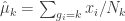
(def cluster-centroids 
  (matrix 
    (for [x_k (group-by training 1 :cols (range 2 12))]
      (map mean (trans x_k)))))

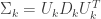
Finally, estimate the covariance matrix to be used for all clusters,

(eq 4.10d) \hat\Sigma=\sum_{k=1}^K\sum_{g_i=k}(x_i-\hat\mu_k)(x_i-\hat\mu_k)^T/(N-K) 
(def cluster-cov-mat 
  (let [groups (group-by training 1 :cols (range 2 12))]
    (reduce plus
      (map (fn [group centroid n]
        (reduce plus 
                (map #(div 
                        (mmult (trans (minus % centroid))
                               (minus % centroid))
                        (- N K))
                     group)))
             groups cluster-centroids group-counts))))

and its inverse:

(def inv-cluster-cov-mat (solve cluster-cov-mat))

With the parameters estimated, now define the linear discriminant function based on equation 4.10 from EoSL:

(eq 4.10) \delta_{k}(x)=x^T\Sigma^{-1}\mu_k-\frac{1}{2}\mu_k^T\Sigma^{-1}\mu_k+log\pi_k  
(defn ldf [x Sigma-inv mu_k pi_k]
  (+ (mmult x Sigma-inv (trans mu_k))
     (- (mult 1/2 (mmult mu_k Sigma-inv (trans mu_k))))
     (log pi_k)))

Differences in the equation, as implemented in the code, and equation 4.10 are because most of the arguments to the ldf function above are row vectors, instead of the column vectors used in eq 4.10.

Next, define a function that returns a matrix of linear discriminate scores, where rows are observations and columns are classes,

(defn calculate-scores
  ([data inv-cov-mat centroids priors]
    (matrix 
      (pmap (fn [row]
             (pmap (partial ldf row inv-cov-mat) 
                   centroids 
                   priors))
           (sel data :cols (range 2 12))))))

and calculate the scores for the training data

(def training-lda-scores 
  (calculate-scores training
                    inv-cluster-cov-mat
                    cluster-centroids
                    prior-probs))

Now, create a function that returns the index (i.e. class) with the maximum score for a given row (i.e. observation) of the scoring matrix,

(defn max-index 
  ([x] 
    (let [max-x (reduce max x)
          n (length x)]
      (loop [i 0]
        (if (= (nth x i) max-x)
          i
          (recur (inc i)))))))

We can get a vector of the predicted class for every observation in the training set with the following line of code:

(map max-index training-lda-scores)

To determine the error rate of the classifier, create the following function,

(defn error-rate [data scores] 
  (/ (sum (map #(if (= %1 %2) 0 1) 
               (sel data :cols 1) 
               (plus 1 (map max-index scores))))
     (nrow data)))

and apply it to the score matrix for the training data,

(error-rate training training-lda-scores)

which returns an error rate of 0.316.

Now let’s see how the classifier performs on the test data. Start by calculating the linear discriminant score matrix,

(def testing-lda-scores 
  (calculate-scores testing
                    inv-cluster-cov-mat
                    cluster-centroids
                    prior-probs))

and then calculate the error-rate,

(error-rate testing testing-lda-scores)

which is 0.556. As expected the error rate is higher on the test data than the training data.

Implementing the QDA Classifier

In order to use QDA to classify the data, we need to estimate a unique covariance matrix for each of the K classes, and write the quadratic discriminant function.

First, estimate the covariance matrices,

(eq 4.10e) \hat\Sigma_k=\sum_{g_i=k}(x_i-\hat\mu_k)(x_i-\hat\mu_k)^T/(N_k-1) 
(def cluster-cov-mats 
  (let [groups (group-by training 1 :cols (range 2 12))]
    (map (fn [group centroid n]
      (reduce plus 
              (map #(div 
                      (mmult (trans (minus % centroid))
                             (minus % centroid))
                      (dec n))
                   group)))
           groups cluster-centroids group-counts)))

and their inverses.

(def inv-cluster-cov-mats (map solve cluster-cov-mats))

Next, create a function that implements the quadratic discriminant function:

(eq 4.12) \delta_{k}(x)=-\frac{1}{2}log|\Sigma_{k}|-\frac{1}{2}(x-\mu_k)^T\Sigma_{k}^{-1}(x-\mu_k)+log\pi_k 
(defn qdf [x Sigma_k Sigma-inv_k mu_k pi_k]
  (+ (- (mult 1/2 (log (det Sigma_k))))
     (- (mult 1/2 (mmult (minus x mu_k) 
                         Sigma-inv_k 
                         (trans (minus x mu_k)))))
     (log pi_k)))

Then calculate the quadratic discriminant score matrix and error rates for the training and test data, which are 0.0113 and 0.528 respectively. Notice that the error rate is substantially lower on the training data than it was with LDA (0.316), but the error rate on the test data is not much better than that achieved by LDA (0.556).

Improving Performance

Hastie, Tibshirani, and Friedman suggested performance of the calculations can be improved by first performing an Eigenvalue decomposition of the covariance matrices.

\Sigma_k=U_kD_kU_k^T 

where U_k is the matrix of eigenvectors, and D_k is a diagonal matrix of positive eigenvalues d_{kl} .

(def Sigma-decomp 
  (map decomp-eigenvalue cluster-cov-matrices ))
(def D (map #(diag (:values %)) Sigma-decomp))
(def U (map #(:vectors %) Sigma-decomp))

Making the following substitutions to \delta_k(x) ,

(a) (x-\hat\mu_k)^T\hat\Sigma_k^{-1}(x-\hat\mu_k)=[U_k^T(x-\hat\mu_k)]^TD_k^{-1}[U_k^T(x-\hat\mu_k)] 
(b) log|\hat\Sigma_k|=\sum_l log(d_{kl}) 

results in the following quadratic discriminant function:

(eq 4.12) \delta_{k}(x)=-\frac{1}{2}\sum_l log(d_{kl})-\frac{1}{2}[U_k^T(x-\hat\mu_k)]^TD_k^{-1}[U_k^T(x-\hat\mu_k)]+log\pi_k 
(defn qdf [x D_k U_k mu_k pi_k]
  (+ (- (mult 1/2 (sum (map log (diag D_k)))))
     (- (mult 1/2 
              (mmult (trans (mmult (trans U_k) 
                                   (trans (minus x mu_k))))
                     (solve D_k) 
                     (mmult (trans U_k) 
                            (trans (minus x mu_k))))))
     (log pi_k)))

This version of the quadratic discriminant function is a bit faster than the previous version, while producing the exact same results. The performance improvement should be greater with larger data sets.

The complete code for this post can be found here.

Incanter Development Roadmap

I want to discuss plans for future Incanter development, and I’m looking for volunteers interested in contributing to any of the following projects, as well as suggestions for other improvements.

My list of priorities, in no particular order:

1. Create new functions based on the Java libraries already included in Incanter. For instance, I would like to improve incanter.optimize by a) including the nonlinear optimization routines available in Parallel Colt b) writing new routines in Clojure, and c) improving the existing routines.

2. Integrate Parallel Colt’s sparse matrix support, as suggested by Mark Reid.

3. Expose more of the chart customizability of JFreeChart in the incanter.chart library, e.g. enabling annotations of categorical charts, allowing users to set the scale on axes, customizing colors, etc..

4. Create an incanter.viz library, consisting of Processing-based data visualizations.

5. Integrate the Weka machine learning library.

6. Provide additional statistical methods.

7. Optimize existing functions; in general, I have favored ease-of-use and expressibility over performance, but there is A LOT of room to optimize without compromising usability.

Any other suggestions or feedback is welcome, and should be directed to the Incanter Goolge Group, where I have started an “Incanter Roadmap” thread. You can subscribe to the mailing list here.

David

Creating Processing Visualizations with Clojure and Incanter

The Processing language, created by Ben Fry and Casey Reas,
“is an open source programming language and environment for people who want to program images, animation, and interactions.”

Incanter now includes the incanter.processing library, a fork of Roland Sadowski‘s clj-processing library, making it possible to create Processing visualizations with Clojure and Incanter. Incanter.processing provides much more flexibility when creating customized data visualizations than incanter.charts — of course, it is also more complex to use.

Several nice examples of the kinds of visualizations that can be created in Processing can be found on Ben Fry’s website and blog, including the cool zipcode, human vs. chimps, baseball salary vs. performance examples.

The processing website has a set of tutorials, including one on getting started, and there are also three great books on Processing worth checking out:

The API documentation for incanter.processing is still a bit underdeveloped, but is perhaps adequate when combined with the excellent API reference on the Processing website.

Incanter.processing was forked from of Roland Sadowski’s clj-processing library in order to provide cleaner integration with Incanter. I have added a few functions, eliminated some, and changed the names of others. There were a few instances where I merged multiple functions (e.g. *-float, *-int) into a single one to more closely mimic the original Processing API; I incorporated a couple functions into Incanter’s existing multi-methods (e.g. save and view); I eliminated a few functions that duplicated existing Incanter functions and caused naming conflicts (e.g. sin, cos, tan, asin, acos, atan, etc); and I changed the function signatures of pretty much every function in clj-processing to require the explicit passing of the ‘sketch’ (PApplet) object, whereas the original library passes it implicitly by requiring that it is bound to a variable called *applet* in each method of the PApplet proxy.

These changes make it easier to use Processing within Incanter, but if you just want to write Processing applications in Clojure without all the dependencies of Incanter, then the original clj-processing library is the best choice.

A Simple Example

The following is sort of a “hello world” example that demonstrates the basics of creating an interactive Processing visualization (a.k.a sketch), including defining the sketch’s setup, draw, and mouseMoved methods and representing state in the sketch using closures and refs. This example is based on this one, found at John Resig‘s Processing-js website.


Click on the image above to see the live Processing-js version of the sketch.

Start by loading the incanter.core and incanter.processing libraries,

(use '(incanter core processing))

Now define some refs that will represent the state of the sketch object,

(let [radius (ref 50.0)
      X (ref nil)
      Y (ref nil)
      nX (ref nil)
      nY (ref nil)
      delay 16

The variable radius will provide the value of the circle’s radius; X and Y will indicate the location of the circle; and nX and nY will indicate the location of the mouse. We use refs for these values because their values are mutable and need to be available across multiple functions in the sketch object.

Now define a sketch object, which is just a proxied processing.core.PApplet, and its required setup method,

sktch (sketch
        (setup []
          (doto this
            (size 200 200)
            (stroke-weight 10)
            (framerate 15)
            smooth)
          (dosync
            (ref-set X (/ (width this) 2))
            (ref-set Y (/ (width this) 2))
            (ref-set nX @X)
            (ref-set nY @Y)))

The first part of the setup method sets the size of the sketch, the stroke weight to be used when drawing, the framerate of the animation, and indicates that anti-aliasing should be used. The next part of the method uses a dosync block and ref-set to set initial values for the refs. Note the @ syntax to dereference (access the values of) the refs X and Y.

Processing sketches that use animation require the definition of a draw method, which in this case will be invoked 15 times per second as specified by the framerate.

  (draw []
   (dosync
     (ref-set radius (+ @radius 
                        (sin (/ (frame-count this) 4))))
     (ref-set X (+ @X (/ (- @nX @X) delay)))
     (ref-set Y (+ @Y (/ (- @nY @Y) delay))))
   (doto this
     (background 125) ;; gray
     (fill 0 121 184)
     (stroke 255)
     (ellipse @X @Y @radius @radius)))

The first part of the draw method uses dosync and ref-set to set new values for the radius, X, and Y refs for each frame of the animation. The sin function is used to grow and shrink the radius over time. The location of the circle, as indicated by X and Y, is determined by the mouse location (nX and nY) with a delay factor.

The next part of the draw method draws the background (i.e. gray background) and the circle with the ellipse function.

Finally, we need to define the mouseMoved method in order to track the mouse location, using the mouse-x and mouse-y functions, and set the values of the nX and nY refs. All event functions in incanter.processing, including mouseMoved, require an event argument; this is due to limitations of Clojure’s proxy macro, and isn’t required when using the Processing’s Java API directly.

(mouseMoved [mouse-event]
  (dosync
    (ref-set nX (mouse-x mouse-event)) 
    (ref-set nY (mouse-y mouse-event)))))]

Now that the sketch is fully defined, use the view function to display it,

(view sktch :size [200 200]))

The complete code for this example can be found here.

In future posts I will walk through other examples of Processing visualizations, some of which can be found in the Incanter distribution under incanter/examples/processing.

Bootstrapping: estimating confidence intervals, standard errors, and bias

In addition to discovering Benford’s law (which I used in a previous post) 57 years before Frank Benford, Simon Newcomb made a series of measurements of the speed of light. In 1882 he measured the time in seconds that a light signal took to travel the 7,400 meters from the US Naval observatory, on the Potomac River, to a mirror at the base of the Washington Monument and back. Newcomb’s data are frequently used to demonstrate statistical techniques, as I will do here. The data are coded as deviations from 24,800 nanoseconds, so the first entry, corresponding to 24,828 nanoseconds, is 28.

Here’s a vector, x, containing the measurements.

(def x [28 -44 29 30 24 28 37 32 36  
        27 26 28 29 26 27 22 23 20  
        25 25 36 23 31 32 24 27 33  
        16 24 29 36 21 28 26 27 27  
        32 25 28 24 40 21 31 32 28  
        26 30 27 26 24 32 29 34 -2  
        25 19 36 29 30 22 28 33 39  
        25 16 23])

There are two obvious outliers in the data, so the median, not the mean, is the preferred estimate of location. Bootstrapping is a method often employed for estimating confidence intervals, standard errors, and estimator bias for medians.

Load the necessary Incanter libraries,

(use '(incanter core stats charts))

View a histogram of the data, note the two outlier observations at -2 and -44.

(view (histogram x 
                 :nbins 20
                 :title "Newcomb's speed of light data"))

Now calculate the median of the sample data

(median x)

The result is 27, but how does this value relate to the speed of light? We can translate this value to a speed in meters/sec with the following function.

(defn to-speed 
  "Converts Newcomb's data into speed (meters/sec)"
  ([x] (div 7400 (div (plus 24800 x) 1E9))))

Now apply it to the median.

(to-speed (median x))

The result is 2.981E8 m/sec (the true speed-of-light is now considered 2.9799E8 m/sec), but how good of an estimate of the median is this? How much sampling error is there? We can estimate confidence intervals, standard errors and estimator bias using bootstrapping.

Bootstrapping is a technique where items are drawn from a sample, with replacement, until we have a new sample that is the same size as the original. Since each item is replaced before the next item is drawn, a single value may appear more than once, and other items may never appear at all. The desired statistic, in this case median, is calculated on the new sample and saved. This process is repeated until you have the desired number of sample statistics. Incanter’s bootstrap function can be used to perform this procedure.

Draw 10,000 bootstrapped samples of the median.

(def t* (bootstrap x median :size 10000))

View a histogram of the bootstrap sample of the median

(view (histogram t* 
                 :density true 
                 :nbins 20
                 :title "Bootstrap sample of medians"
                 :x-label "median"))

The bootstrap distribution is very jagged because the median is discrete, so there are only a small number of values that it can take. Later, I will demonstrate how to smooth over the discreteness of the median with the :smooth option to the bootstrap function.

The mean of t* is the bootstrap estimate of the median,

(mean t*)

which is 27.301. An estimate of the 95% confidence interval (CI) for the median can be calculated with the quantile function.

(quantile t* :probs [0.025 0.975])

The CI is estimated as (26.0 28.5). The standard error of the median statistic is estimated by the standard deviation of the bootstrap sample.

(sd t*)

The standard error estimate is 0.681. The bias of the median statistic is estimated as the difference between it and the mean of the bootstrap sample.

(- (mean t*) (median x))

The estimator bias is -0.3.

Smoothing

As was apparent in the previous histogram, the bootstrap distribution is jagged because the median is discrete. In order to smooth over the discreteness of the median, we can add a small amount of random noise to each bootstrap sample. The :smooth option adds gaussian noise to each median in the sample. The mean of the noise equals zero and the standard deviation equals 1/sqrt(n), where n is the original sample size.

Draw 10000 smoothed bootstrap samples of the median

(def smooth-t* (bootstrap x median 
                          :size 10000 
                          :smooth true))

View a histogram of the smoothed bootstrap samples of the median

(view (histogram smooth-t* 
                 :density true 
                 :nbins 20
                 :title "Smoothed bootstrap sample of medians"
                 :x-label "median"))

Calculate the estimate of the median.

(mean smooth-t*)

The smoothed estimate of the median is 27.304. Now, calculate a 95% CI.

(quantile smooth-t* :probs [0.025 0.975])

The smoothed result is (25.905 28.446).

The complete code for this example can be found here.

Bayesian inference of multinomial distribution parameters

The multinomial distribution is used to describe data where each observation is one of k possible outcomes. In his book, Bayesian Data Analysis (pg 83), Andrew Gelman demonstrates how to use Bayesian methods to make inferences about the parameters of a multinomial distribution. He used data from a sample survey by CBS news prior to the 1988 presidential election. In his book Bayesian Computation with R (pg. 60), Jim Albert used R to perform the same inferences on the same data as Gelman. I’ll now demonstrate how to perform these inferences in Clojure, with Incanter, using the sample-multinomial-params function. I will then describe the Bayesian model underlying sample-multinomial-params, and demonstrate how to do the same calculations directly with the sample-dirichlet function.

First, load the necessary libraries, including the incanter.bayes library.

(use '(incanter core stats bayes charts))

The data consist of 1447 survey responses; 727 respondents supported George Bush Sr., 583 supported Michael Dukakis, and 137 supported another candidate, or were undecided. Define a vector, y, that includes the counts for each of the outcomes.

(def y [727 583 137])

The proportion of supporters for the candidates, calculated by dividing y by the total responses,

(div y 1447)

are (0.502 0.403 0.095). If the survey data follows a multinomial distribution, these proportions are the parameters of that distribution. The question is, how good an estimate of the population parameters are these values?

Confidence intervals for the parameters can be calculated by applying the quantile function to a sample drawn from an appropriate distribution, which in the case of the parameters of a multinomial distribution is a Dirichlet distribution.

Samples can be drawn from the appropriate Dirichlet distribution with the sample-multinomial-params function.

(def  theta (sample-multinomial-params 1000 y))

This returns 1000 samples of the multinomial parameters, or probabilities of each of the outcomes in the data. Now, create variables representing the samples for each parameter,

(def theta1 (sel theta :cols 0))
(def theta2 (sel theta :cols 1))
(def theta3 (sel theta :cols 2))

and calculate the mean, standard deviation, 95% confidence interval, and display a histogram for each sample.

(mean theta1)
(sd theta1)
(quantile theta1 :probs [0.025 0.975]) 
(view (histogram theta1
                 :title "Bush, Sr. Support"))

The mean for theta1 is 0.502, the standard deviation is 0.013, and the 95% confidence interval is (0.476 0.528).

(mean theta2) 
(sd theta2)
(quantile theta2 :probs [0.025 0.975]) 
(view (histogram theta2
                 :title "Dukakis Support"))

The mean for theta2 is 0.403, the standard deviation is 0.013, and the 95% confidence interval is (0.376 0.427).

(mean theta3) 
(sd theta3)
(quantile theta3 :probs [0.025 0.975]) 
(view (histogram theta3
                 :title "Other/Undecided"))

The mean for theta3 is 0.095, the standard deviation is 0.008, and the 95% confidence interval is (0.082 0.111).

Using the sample distributions for the parameters, we can view the distribution of other statistics, like the difference in support between Bush, Sr. and Dukakis. View a histogram of the difference in support for the two candidates.

(view (histogram (minus theta1 theta2) 
                 :title "Bush, Sr. and Dukakis Diff"))

The sample-multinomial-params functions returns values from a Dirichlet distribution. The Dirichlet is the conjugate prior distribution for the parameters of the multinomial distribution, such that the posterior Dirichlet’s parameters equal the sum of the count data, y, and the parameters from the prior Dirichlet, alpha.

 p(\theta | y+\alpha) = p(y | \theta)p(\alpha)/p(y)  

Where

 y = (y_1, y_2, ..., y_k)  

are the count data that follow a multinomial distribution,

 \theta = (\theta_1, \theta_2, ..., \theta_k)  

are the parameters of the multinomial distribution, and

 \alpha = (\alpha_1, \alpha_2, ..., \alpha_k)  

are the hyper-parameters of the prior Dirichlet distribution. The likelihood function, p(y | theta), is a multinomial conditional distribution that describes the likelihood of seeing the observed y values, given the values of the parameter, theta.

The prior, p(alpha), is made uninformative by setting all the alpha values equal to one, producing a uniform distribution.

 \alpha = (1, 1, ..., 1) 

Then the posterior Dirichlet becomes

 p(\theta | y_1+1, y_2+1, .., y_3+1)  

Sample the proportions directly from the above Dirichlet distribution using the sample-dirichlet function.

(def alpha [1 1 1])
(def  props (sample-dirichlet 1000 (plus y alpha)))

This returns data from the same distribution as the sample-multinomial-params function, so all the means, standard deviations, and confidence intervals can be calculated as above.

The complete code for this example is here.

Monty Hall in Monte Carlo

The Monty Hall problem, named after the host of the Let’s Make a Deal game show, first appeared in Marilyn vos Savant‘s column in Parade magazine in 1990, although people still vigorously debate the answer, as discussed here and here.

The basic premise is that you must choose one of three doors, one of which contains a prize. Once you have selected a door, Monty Hall reveals the contents of one of the doors you did not select, usually containing something like a goat. He then asks if you would like to switch your choice to the remaining unopened door. The question is, will switching doors increase you chances of winning, decrease your chances, or have no effect at all?

One thing to keep in mind, is that when Monty Hall shows you what’s behind one of the doors you didn’t select, he doesn’t ever reveal the door containing the prize. This fact should change your decision making process.

We can answer the question of which strategy is best by calculating the conditional probabilities of winning given you either switch or stay by performing a Monte Carlo simulation. The conditional probability of winning given you decide to switch doors can be written as Prob(win | switch), and is equal to the probability that you switch and win divided by the probability that you switch,

Prob(win | switch) = Prob(switch & win)/Prob(switch)

and the conditional probability of winning given you decide to stay with your original door is equal to the probability you stay and win divided by the probability that you stay.

Prob(win | stay) = Prob(stay & win)/Prob(stay)

In this simulation, we will generate a bunch of initial guesses, a bunch of prize locations, and a bunch of switch decisions and then use them to calculate the probabilities. First, load the necessary libraries.

(use '(incanter core stats charts))

Set a simulation sample size, generate samples of initial-guesses, prize-doors, and switch decisions with the sample function. The probability that the prize is behind any of the three doors is 1/3, as is the probability that you select a particular door as an initial guess, while the probability that you switch doors is 1/2.

(def n 10000)
(def initial-guesses (sample [1 2 3] :size n))
(def prize-doors (sample [1 2 3] :size n))
(def switches (sample [true false] :size n))

Define a function that returns one if a switch decision results in winning, a zero otherwise.

(defn switch-win? [initial-guess switch prize-door] 
  (if (and switch (not= initial-guess prize-door)) 1 0))

Calculate the joint probability of winning and switching, by mapping the switch-win? function over the generated data, summing the occurrences of winning after switching, and then dividing this number by the total number of samples, n.

(def prob-switch-win (/ (sum (map switch-win? 
                              initial-guesses 
                              switches 
                              prize-doors)) 
                        n))

Calculate the probability of switching doors. Use the indicator and sum functions to calculate the frequency of switches, and then divide by the total number of samples.

(def prob-switch (/ (sum (indicator true? switches)) n))

Finally, use the formula above to calculate the conditional probability of winning given a switch.

(def prob-win-given-switch (/ prob-switch-win prob-switch))

Now repeat the process to calculate the conditional probability of winning given the decision to stay with your original choice. First, define a function that returns a one if a stay decision results in winning, zero otherwise.

(defn stay-win? [initial-guess switch prize-door] 
  (if (and (not switch) (= initial-guess prize-door)) 1 0))

Next, calculate the joint probability of winning and staying,

(def prob-stay-win (/ (sum (map stay-win? 
                            initial-guesses 
                            switches 
                            prize-doors)) 
                      n))

and, calculate the probability of staying with the original door.

(def prob-stay (/ (sum (indicator false? switches)) n))

Finally, calculate the conditional probability of winning given you stay with the original door

(def prob-win-given-stay (/ prob-stay-win prob-stay))

View the results with the pie-chart function.

(view (pie-chart ["Switch" "Stay"] 
                 [prob-win-given-switch prob-win-given-stay]))

The conditional probability of winning given you switch doors is approximately 0.66, while the probability of winning given you stay with your original choice is approximately 0.33.

To some this outcome may seem non-intuitive. Here’s why it’s the case: the probability that the prize is behind any of the three doors is 1/3, so once you have selected a door, the probability that the prize is behind a door you didn’t select is 2/3. Since Monty Hall knows which door has the prize, and never selects it as the door to reveal, all of the 2/3 probability belongs to the other unselected door. So switching will give you a 2/3 probability of winning the prize, and sticking with your original decision only gives you the original 1/3 chance.

The complete code for this example can be found here.

Chi-square goodness-of-fit, Benford’s law, and the Iranian election

Benford’s law has been discussed as a means of analyzing the results of the 2009 Iranian election by several analysts. One of the first attempts was in a paper (pdf) by Boudewijn Roukema, where he concluded that the data did not follow Benford’s law, and that there was evidence for vote tampering. Andrew Gelman responded; he was not convinced by the statistics of this particular analysis (his criticism was of the statistical analysis, and didn’t reflect his opinion of the possibility of vote tampering).

Stochastic Democracy and the Daily Kos also used Benford’s law to analyze the election data, here, but came to the opposite conclusion of Roukema; the data did follow Benford’s law. A third analysis was performed by John Graham-Cumming in this blog post. He came to the same conclusion as Stochastic Democracy and Daily Kos, that the data did follow Benford’s law. His analysis is based on this data, available from the Guardian’s Data Blog.

Again, like Gelman, I’m not convinced that Benford’s law can necessarily be used to draw conclusions on the presence or absence of vote tampering, but it is an interesting example of a Chi-square goodness-of-fit analysis, comparing some real-world data with a theoretical distribution, Benford’s law in this case. So I will demonstrate how to perform the analysis with Incanter using the data set made available by the Guardian. A CSV file with the data can be found here.

First load the necessary libraries,

(use '(incanter core stats charts io))

and read the data using the read-dataset function.

(def votes (read-dataset "data/iran_election_2009.csv" 
                         :header true))

Now, create variables representing the regions and the candidates.

(def regions (sel votes :cols "Region"))
(def ahmadinejad-votes (sel votes :cols "Ahmadinejad"))
(def mousavi-votes (sel votes :cols "Mousavi"))
(def rezai-votes (sel votes :cols "Rezai"))
(def karrubi-votes (sel votes :cols "Karrubi"))

We need to write a small function that will take a number and return only the first digit. We can do that by converting the number into a string with the str function, taking the first character of the string, and then converting that character into a number again.

(defn first-digit [x] 
  (Character/digit (first (str x)) 10)) 

Now, map the first-digit function over the vote counts in each of the 30 regions for each candidate.

(def ahmadinejad (map first-digit ahmadinejad-votes))
(def mousavi (map first-digit mousavi-votes))
(def rezai (map first-digit rezai-votes))
(def karrubi (map first-digit karrubi-votes))

Now we have a list of first-digits across the different regions, for each candidate. Next, define function that implements Benford’s Law, create a variable containing the probabilities for each of the nine digits, and calculate the expected frequencies for the 30 regions.

(defn benford-law [d] (log10 (plus 1 (div d))))
(def benford-probs (benford-law (range 1 11)))
(def benford-freq (mult benford-probs (count regions)))

We will then need a function that takes the list of first digits for each candidate and returns the counts for each digit. We can use the :counts field returned by the tabulate function to do most of the work.

(defn get-counts [digits] 
  (map #(get (:counts (tabulate digits)) % 0) 
       (range 1.0 10.0 1.0)))

It’s always a good idea to look at the data, so plot the predicted first-digit frequencies and the frequencies for Ahmadinejad and Mousavi.

(doto (xy-plot (range 1 10) (get-counts ahmadinejad)
               :legend true :series-label "Ahmadinejad"
               :y-label "First digit frequency"
               :x-label "First digit"
               :title "First digit frequency by candidate")
      (add-lines (range 1 10) (get-counts mousavi) 
                 :series-label "Mousavi")
      (add-lines (range 1 10) benford-freq 
                 :series-label "Predicted")
      clear-background
      view)

Based on that plot, the digit frequencies look like they follow Benford’s law. We can confirm that with a Chi-square goodness-of-fit test using the chisq-test function. Start with Ahmadinejad,

(def ahmadinejad-test 
  (chisq-test :table (get-counts ahmadinejad) 
              :probs benford-probs))
(:X-sq ahmadinejad-test)
(:p-value ahmadinejad-test)

The X-square test value is 5.439 with a p-value of 0.71. Based on these values we cannot reject the null hypothesis that the observed distribution of first-digits is the same as the expected distribution, which follows Benford’s law. Next test Mousavi’s vote counts,

(def mousavi-test 
  (chisq-test :table (get-counts mousavi) 
              :probs benford-probs))
(:X-sq mousavi-test) 
(:p-value mousavi-test)

The X-square test value for Mousavi is 5.775 with a p-value of 0.672. Like Ahmadinejad, we cannot reject the null hypothesis. We might as well test the distributions of first-digits for the remaining two candidates (which we didn’t plot), Rezai and Karrubi.

(def rezai-test 
  (chisq-test :table (get-counts rezai) 
              :probs benford-probs))
(:X-sq rezai-test) 
(:p-value rezai-test) 

The X-square test value for Rezai is 12.834 with a p-value of 0.118, so we can’t reject the null hypothesis.

(def karrubi-test 
  (chisq-test :table (get-counts karrubi) 
              :probs benford-probs))
(:X-sq karrubi-test) 
(:p-value karrubi-test) 

Karrubi’s X-square value is 8.8696 with a p-value of 0.353, and like the other candidates appears to follow Benford’s law.

The conclusion based on the vote count summaries for the 30 Iranian regions, is that the votes follow Benford’s law.

Last-digit frequencies

Another approach to identifying vote tampering is to examine the last digit of the vote counts, instead of the first. This approach was discussed in this Washington Post article.

Unlike first-digits, last-digits don’t follow Benford’s law, but rather follow a uniform distribution. We can test the distribution of last-digits from our sample of 30 regions using the chisq-test function again. First, define a function to extract the last digit from a number,

(defn last-digit [x] 
  (Character/digit (last (str x)) 10))

and map the function over the vote counts for each candidate.

(def ahmadinejad-last (map last-digit 
                           ahmadinejad-votes))
(def mousavi-last (map last-digit 
                       mousavi-votes))
(def rezai-last (map last-digit 
                     rezai-votes))
(def karrubi-last (map last-digit 
                       karrubi-votes))

Now we have a list of last-digits for the 30 regions for each candidate. We need to tweak the get-counts function, from above, so that it includes the digit zero, which wasn’t necessary in the first-digit case.

(defn get-counts [digits] 
  (map #(get (:counts (tabulate digits)) % 0) 
       (range 0.0 10.0 1.0)))

Now plot the last-digit distribution for each of hte candidates.

(doto (xy-plot (range 10) 
               (get-counts ahmadinejad-last)
               :legend true 
               :series-label "Ahmadinejad"
               :y-label "First digit frequency"
               :x-label "First digit"
               :title "Last digit frequency by candidate")
      (add-lines (range 10) (get-counts mousavi-last) 
                 :series-label "Mousavi")
      (add-lines (range 10) (get-counts rezai-last) 
                 :series-label "Rezai")
      (add-lines (range 10) (get-counts karrubi-last) 
                 :series-label "Karrubi")
      clear-background
      view)

The data certainly doesn’t look like it’s following Benford’s law, but is it uniformly distributed? We can test that hypothesis with the chisq-test function, this time we won’t need to supply the :probs argument because a uniform distribution is the default.

(def ahmadinejad-test 
  (chisq-test :table (get-counts ahmadinejad-last)))

(:X-sq ahmadinejad-test) ;; 4.667
(:p-value ahmadinejad-test) ;; 0.862

(def mousavi-test 
  (chisq-test :table (get-counts mousavi-last)))
(:X-sq mousavi-test) ;; 8.667
(:p-value mousavi-test) ;; 0.469

(def rezai-test 
  (chisq-test :table (get-counts rezai-last)))
(:X-sq rezai-test) ;; 15.333 
(:p-value rezai-test) ;; 0.0822

(def karrubi-test 
  (chisq-test :table (get-counts karrubi-last)))
(:X-sq karrubi-test) ;; 4.0
(:p-value karrubi-test) ;; 0.911

According to each of these tests, we cannot reject the hypothesis that the last-digits for each candidate follows a uniform distribution. The analysis written up in the Washington Post article came to the opposite conclusion, which is likely due to their use of more detailed data. The data used here was summary information for 30 regions. More detailed vote counts could certainly provide a different conclusion.

The complete code for this post can be found here.